47.269 Research I:  Basics

Inferential Statistics & Hypothesis Testing

Beyond Description

First, go back to what we learned in Chapter 3 and on pp. 437-467 of Chapter 15.  Once you have had a chance to review that, think about how those two lessons relate to those sections of Chapter 15 that you are reading for this week. 

Basically, you have the concepts involved in inferential statistics.  Now all we are going to do is formalize them just the least little bit.  You will go into much, much more in Research II and III.

Okay, important review concepts are these:

· Level of data

· Samples vs. Populations

· Descriptive sample statistics (estimates) vs. Population parameters

· Central tendency

· Variability

· Differences within vs. Differences between

· Size of the study & the law of large numbers

Recall the null hypothesis compared with the experimental hypopthesis.  What is important to remember is that when we go beyond simply describing our data (e.g., proportions or means and standard deviations) and we try to make an inference about what they mean with respect to the population, we can only infer with respect to the null hypothesis.

In other words, we don’t find data to “prove” the alternative or experimental hypothesis, we look for just enough evidence to reject the null.

It’s the old double negative:

o reject the nullà

o reject no difference à

o not no difference

o By default then, we assume there is a difference

o But, we have not proven there is a difference

When we are comparing two groups with scores at more than a nominal level—say, the scores of boys and girls on a standardized test of mathematics—we start off assuming they are not different.

What does that mean? It means that we assume our sample of boys and girls are drawn from the SAME population distribution of math scores.

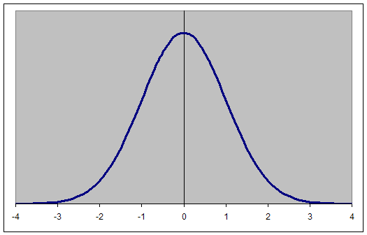
Picture the normal curve (i.e., the bell shaped curve).  Assuming boys and girls came from the SAME population of scores, there would be a high likelihood of getting scores from the clump in the middle when we randomly selected a sample of boys and a sample of girls.

Standard Normal Distribution

Mean = 0, SD = 1

So the boy scores and girl scores in the samples might not be exactly the same, but they should be close. 

What does close mean?  Think back to previous lectures.  It means that the difference between the boy and girl scores is no bigger than the differences (or variability) within the boys’ scores and within the girls’ scores.

If, on the other hand, the girls’ scores started clustering around -1 SD on the distribution above and the boys’ started clustering around +1 SD… well, what would that mean???

· It might be a statistical fluke, since there is a chance that you could randomly select children whose scores just so happened to be there

§ How big was your sample? The smaller it is, the more likely you could get such a fluke.  The larger it is, the more likely you are getting a sample representative of the population and not just some bizarre unusual chance thing

· It could mean that the boys and girls were really different populations with respect to their math scores, with boys having a slightly higher mean (i.e., peak to their normal curve) and girls having a slightly lower one.

§ Again, how big is your sample? How confident are you that it represents the population well?  The bigger the sample, the more confident you can be.  In other words, the bigger your sample, the smaller your sampling error. (see p. 404)

So, what to do with these scores?? 

First, plot them.  Compare their bar charts or frequency distributions to each other. What do these pictures tell you?

Now get a number to quantify that visual message and test your hypothesis.

As your book says (p. 440) the hypothesis test is a procedure that evaluates sample data by computing statistics to bring evidence to the credibility of a hypothesis by distinguishing whether patterns in the data

· Represent REAL relations among variables in the population

§ OR

· Are simply due to chance, i.e., sampling error

In other words, given the size of your samples and the patterns in the scores, how reasonable is it that you could have just so happened to pick these participants if in fact both groups came from the same population?

One way to think about that question is to ask:  How likely would I be to get the same results if I tried it again?

And just to be really sure, Again.

And Again.

And Again.

And….Well, you get the picture.

Inferential statistics are based on the idea that we calculate how often such a pattern would emerge in the data IF the data from two or more groups all came from the same normally distributed population.

If it is an unusual, once in a blue moon event, we assume that it is much more likely that the groups come from different populations and we reject the null hypothesis.

I mean, what are the odds???  Is it more likely that you pulled from the tiny numbers in the extremes of one distribution OR more likely that you pulled scores from two different clumps in the middle of two different distributions?

In other words, imagine when you get the results for your two groups that you were to randomly sample over and over and over again.  Under the assumption of the null hypothesis, the groups actually come from one population and there is no difference.  So under that assumption, you should get an average scores that, although they vary each time you collect a new sample and will, themselves begin to take the shape of a normal distribution. 

So, if you just so happen to come up with an extreme scores—i.e., not ones in the middle, but ones on the infrequently occurring tails—on your very first try at sampling these two groups, it would be a very unlikely event.

Instead, it is much more likely that you pulled scores from two different clumps in the middle of two different distributions

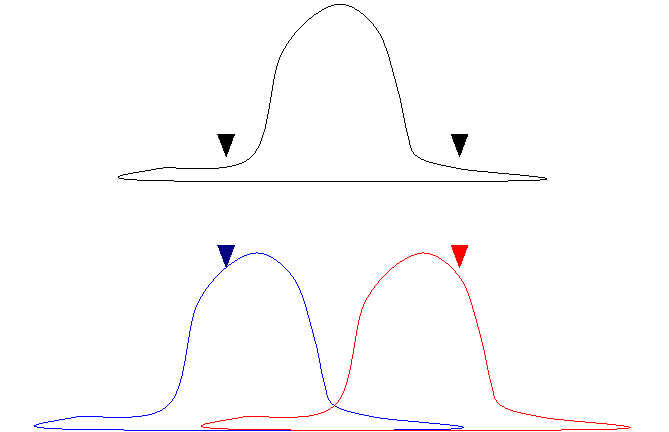
In these free hand representations of normally distributed data, we compare the how likely it would be to get the scores pictured by triangles if they were taken from a single population with how likely it would be if they were taken from two populations, here pictured in red and blue. There are few scores at these places in the top single population example.  There are many scores like these in the two population example.

What do you do then?  Rather than assume this unlikely event happened, you assume the more likely event did and that you actually sampled from two different populations. 

Great.  So we have rejected the null hypothesis, i.e., rejected the idea that there is no real relationship between the variables (gender and math scores, in this case).  Instead we find support for the alternative hypothesis that there is a relation between gender and math, that boys and girls differ in their mathematics performance on standardized tests.

But….

Are you sure?????

No, of course not.  You are placing your bets on the most likely explanation for the data you have obtained.

There is a chance that you will be wrong!

How much of a chance are you willing to take?

            How about a 50% chance?  No? 

                        How about a 0.20 (otherwise known as 20%) chance?  Still too high? 

                                    How about a 5% (or 0.05) chance?  Could you live with that?

Well, it turns out, that the standard risk we take in psychology is the .05 level.  We examine the results and compute our statistics and infer whether we can reject the null hypothesis or not with about a 5% chance that we are making an error in our inference.

This level of chance we are willing to take is called the alpha level (see p. 442-443).  Sometimes we are willing to take a bit more chance, sometimes we can reject the null hypothesis and infer a real relation between the variables with even less of a chance—say .01 or .001.  It all depends on:

· the size of the effect, i.e., the ratio of difference between to difference within, and

· the size of the sample.

Both of these items enter into the equation.  A modest effect size can pair up with a large sample size or a huge effect size in combination with a smaller sample might result in inferences that the observed relations among the variables are real with a degree of certainty, that is, they are statistically significant at a particular alpha level.

Because we do not have certainty, there is always a chance of making a mistake.

· A Type I error occurs when the sample data permit you to infer a relationship when there is really none in the population. 

· Sampling fluke?  This is more likely to happen when you set too high an alpha level.

· A Type II error occurs when the sample data fail to detect a relationship that is really there in the population. 

· Could be too small an alpha level.  Could be too small a sample.

Okay, time out.  Do you get these concepts?  That is all I really want you to do here.  You will build on this significantly in Research II.  For now, we will just push ahead a little bit, but you do not need to understand the intricacies of the inferential statistics we discuss, just their application in principle.