|
Info on Grad
Schools:
Buy Books, CDs, &
Videos:
Digital Camera:
Rio MP3 Player:
Diamond Rio 500 Portable MP3 Player
Memory Upgrade:
$1.23 per issue:
Ebay Auction:
$1.83 per issue: |
Theory of Data Compression
Contents
- Introduction
and Background
- Source
Modeling
- Entropy Rate
of a Source
- Shannon
Lossless Source Coding Theorem
- Rate-Distortion
Theory
- The Gap
Between Theory and Practice
- FAQs
(Frequently Asked Questions)
- References
I. Introduction and
Background
Claude E.
Shannon
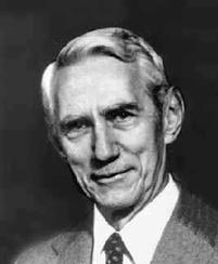 | In his 1948 paper, ``A
Mathematical Theory of Communication,'' Claude E. Shannon formulated
the theory of data compression. Shannon established that there is a fundamental
limit to lossless
data compression. This limit, called the entropy
rate, is denoted by H. The exact value of H depends on
the information source --- more specifically, the statistical
nature of the source. It is possible to compress the source, in a
lossless manner, with compression
rate close to H. It is mathematically impossible to do better
than H.
Shannon also developed the theory of lossy
data compression. This is better known as rate-distortion
theory. In lossy data compression, the decompressed data does not have
to be exactly the same as the original data. Instead, some amount of distortion,
D, is tolerated. Shannon showed that, for a given source (with all
its statistical properties known) and a given distortion
measure, there is a function, R(D), called the rate-distortion
function. The theory says that if D is the tolerable amount of
distortion, then R(D) is the best possible compression rate.
When the compression is lossless (i.e., no distortion or D=0),
the best possible compression rate is R(0)=H (for a finite alphabet
source). In other words, the best possible lossless compression rate is
the entropy rate. In this sense, rate-distortion theory is a
generalization of lossless data compression theory, where we went from no
distortion (D=0) to some distortion (D>0).
Lossless data compression theory and rate-distortion theory are known
collectively as source
coding theory. Source coding theory sets fundamental limits on the
performance of all data compression algorithms. The theory, in itself,
does not specify exactly how to design and implement these algorithms. It
does, however, provide some hints and guidelines on how to achieve optimal
performance. In the following sections, we will described how Shannon
modeled an information source in terms of a random process, we will
present Shannon lossless source coding theorem, and we will discuss
Shannon rate-distortion theory. A background in probability theory is
recommended.
II. Source Modeling
Available at
Amazon.com
 | Imagine that you go to the
library. This library has a large selection of books --- say there are 100
million books in this library. Each book in this library is very thick ---
say, for example, that each book has 100 million characters (or letters)
in them. When you get to this library, you will, in some random manner,
select a book to check out. This chosen book is the information source to
be compressed. The compressed book is then stored on your zip disk to take
home, or transmitted directly over the internet into your home, or
whatever the case may be.
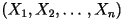
Mathematically, the book you select is denoted by
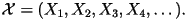 where where  represents the whole book,
  represents the first character in the book,
  represents the second character, and so on. Even though in reality the
length of the book is finite, mathematically we assume that it has
infinite length. The reasoning is that the book is so long we can just
imagine that it goes on forever. Furthermore, the mathematics turn out to
be surprisingly simpler if we assume an infinite length book. To simplify
things a little, let us assume that all the characters in all the books
are either a lower-case letter (`a' through `z') or a SPACE (e. e.
cummings style of writing shall we say). The source
alphabet,
represents the second character, and so on. Even though in reality the
length of the book is finite, mathematically we assume that it has
infinite length. The reasoning is that the book is so long we can just
imagine that it goes on forever. Furthermore, the mathematics turn out to
be surprisingly simpler if we assume an infinite length book. To simplify
things a little, let us assume that all the characters in all the books
are either a lower-case letter (`a' through `z') or a SPACE (e. e.
cummings style of writing shall we say). The source
alphabet,  ,
is defined to be the set of all 27 possible values of the characters: ,
is defined to be the set of all 27 possible values of the characters:
 Now put yourself in the shoes of the
engineer who designs the compression algorithm. She does not know in
advance which book you will select. All she knows is that you will be
selecting a book from this library. From her perspective, the characters
in the book Now put yourself in the shoes of the
engineer who designs the compression algorithm. She does not know in
advance which book you will select. All she knows is that you will be
selecting a book from this library. From her perspective, the characters
in the book 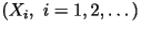 are random
variables which take values on the alphabet .
The whole book,
is just an infinite sequence of random variables -- that is
is a random
process. There are several ways in which this engineer can model the
statistical properties of the book.
are random
variables which take values on the alphabet .
The whole book,
is just an infinite sequence of random variables -- that is
is a random
process. There are several ways in which this engineer can model the
statistical properties of the book.
- Zero-Order Model: Each character is
statistically independent of all other characters and the 27 possible
values in the alphabet
are equally likely to occur. If this model is accurate, then a typical
opening of a book would look like this (all of these examples came
directly from Shannon's
1948 paper):
xfoml rxkhrjffjuj zlpwcfwkcyj ffjeyvkcqsghyd qpaamkbzaacibzlhjqd
This does not look like the writing of an intelligent being. In fact,
it resembles the writing of a ``monkey sitting at a typewriter.''
- First-Order Model: We know that in the
English language some letters occur more frequently than others. For
example, the letters `a' and `e' are more common than `q' and `z'. Thus,
in this model, the character are still independent of one another, but
the probability distribution of the characters are according to the first-order
statistical distribution of English text. A typical text for this
model looks like this:
ocroh hli rgwr nmielwis eu ll nbnesebya th eei alhenhttpa oobttva nah
brl
- Second-Order Model: The previous two
models assumed statistical independence from one character to the next.
This does not accurately reflect the nature of the English language. For
exa#ple, some letters in thi# sent#nce are missi#g. However, we are
still able to figure out what those letters should have been by looking
at the context. This implies that there are some dependency between the
characters. Naturally, characters which are in close proximity are more
dependent than those that are far from each other. In this model, the
present character
 depends on the previous character
  but it is conditionally independent of all previous characters
  . According to this model, the probability distribution of
the character
varies according to what the previous character
is. For example, the letter `u' rarely occurs (probability=0.022).
However, given that the previous character is `q', the probability of a
`u' in the present character is much higher (probability=0.995). For a
complete description, see the second-order
statistical distribution of English text. A typical text for this
model would look like this: . According to this model, the probability distribution of
the character
varies according to what the previous character
is. For example, the letter `u' rarely occurs (probability=0.022).
However, given that the previous character is `q', the probability of a
`u' in the present character is much higher (probability=0.995). For a
complete description, see the second-order
statistical distribution of English text. A typical text for this
model would look like this:
on ie antsoutinys are t inctore st be s deamy achin d ilonasive
tucoowe at teasonare fuso tizin andy tobe seace ctisbe
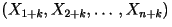
- Third-Order Model: This is an extension
of the previous model. Here, the present character
depends on the previous two characters
 but it is conditionally independent of all previous characters before
those:
but it is conditionally independent of all previous characters before
those:  . In this model, the distribution of varies according to what
are. See the third-order
statistical distribution of English text. A typical text for this
model would look like this: . In this model, the distribution of varies according to what
are. See the third-order
statistical distribution of English text. A typical text for this
model would look like this:
in no ist lat whey cratict froure birs grocid pondenome of
demonstures of the reptagin is regoactiona of cre
The resemblance to ordinary English text increases quite noticeably
at each of the above steps.
- General Model: In this model, the book
is an arbitrary stationary
random process. The statistical properties of this model are too complex
to be deemed practical. This model is interesting only from a
theoretical point of view.
Model A above is a special
case of Model B. Model B is a special case of Model C. Model C is a
special case of Model D. Model D is a special case of Model E.
III. Entropy Rate of a
Source
Shannon in
1948
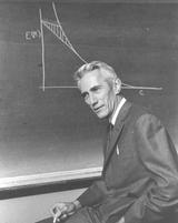 | The entropy rate of a source is a
number which depends only on the statistical nature of the source. If the
source has a simple model, then this number can be easily calculated.
Here, we consider an arbitrary source:
 while paying special attention to the
case where
is English text. while paying special attention to the
case where
is English text.
- Zero-Order Model: The characters are
statistically independent of each other and every letter of the
alphabet,, are equally likely to occur. Let
 be the size of the alphabet. In this case, the entropy rate is given by
 For English text, the alphabet size is
m=27. Thus, if this had been an accurate model for English text,
then the entropy rate would have been H=log2 27=4.75
bits/character. For English text, the alphabet size is
m=27. Thus, if this had been an accurate model for English text,
then the entropy rate would have been H=log2 27=4.75
bits/character.
- First-Order Model: The characters are
statistically independent. Let
be the size of the alphabet and let
 be the probability of the i-th letter in the alphabet. The
entropy rate is
be the probability of the i-th letter in the alphabet. The
entropy rate is
 Using the first-order
distribution, the entropy rate of English text would have been 4.07
bits/character had this been the correct model. Using the first-order
distribution, the entropy rate of English text would have been 4.07
bits/character had this been the correct model.
- Second-Order Model: Let
 be the conditional probability that the present character is the
j-th letter in the alphabet given that the previous character is
the i-th letter. The entropy rate is
be the conditional probability that the present character is the
j-th letter in the alphabet given that the previous character is
the i-th letter. The entropy rate is
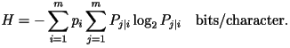 Using the second-order
distribution, the entropy rate of English text would have been 3.36
bits/character had this been the correct model. Using the second-order
distribution, the entropy rate of English text would have been 3.36
bits/character had this been the correct model.
- Third-Order Model: Let
 be the conditional probability that the present character is the
k-th letter in the alphabet given that the previous character is
the j-th letter and the one before that is the i-th
letter. The entropy rate is
be the conditional probability that the present character is the
k-th letter in the alphabet given that the previous character is
the j-th letter and the one before that is the i-th
letter. The entropy rate is
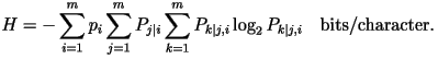 Using the third-order
distribution, the entropy rate of English text would have been 2.77
bits/character had this been the correct model. Using the third-order
distribution, the entropy rate of English text would have been 2.77
bits/character had this been the correct model.
- General Model: Let
 represents the first
  characters. The entropy rate in the general case is given by
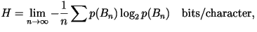 where the sum is over all where the sum is over all  possible values of . It is virtually impossible to calculate the entropy rate
according to the above equation. Using a prediction method, Shannon has
been able to estimate that the entropy rate of the 27-letter English
text is 2.3 bits/character (see Shannon:Collected
Papers). possible values of . It is virtually impossible to calculate the entropy rate
according to the above equation. Using a prediction method, Shannon has
been able to estimate that the entropy rate of the 27-letter English
text is 2.3 bits/character (see Shannon:Collected
Papers). We emphasize that there is only one entropy rate
for a given source. All of the above definitions for the entropy rate are
consistent with one another.
IV. Shannon Lossless Source Coding
Theorem
Excellent
Textbook
 | Shannon lossless source coding
theorem is based on the concept of block coding. To illustrate this
concept, we introduce a special information source in which the alphabet
consists of only two letters:
 Here, the letters `a' and `b' are equally
likely to occur. However, given that `a' occurred in the previous
character, the probability that `a' occurs again in the present character
is 0.9. Similarly, given that `b' occurred in the previous character, the
probability that `b' occurs again in the present character is 0.9. This is
known as a binary symmetric Markov source. Here, the letters `a' and `b' are equally
likely to occur. However, given that `a' occurred in the previous
character, the probability that `a' occurs again in the present character
is 0.9. Similarly, given that `b' occurred in the previous character, the
probability that `b' occurs again in the present character is 0.9. This is
known as a binary symmetric Markov source.
An n-th order block code is just a mapping which assigns to each
block of n consecutive characters a sequence of bits of varying
length. The following examples illustrate this concept.
- First-Order Block Code: Each character is
mapped to a single bit.
 |
 |
Codeword |
| a |
0.5 |
0 |
| b |
0.5 |
1 |
| R=1
bit/character |
An example:

Note that 24 bits are used to
represent 24 characters --- an average of 1 bit/character.
- Second-Order Block Code: Pairs of
characters are mapped to either one, two, or three bits.
 |
 |
Codeword |
| aa |
0.45 |
0 |
| bb |
0.45 |
10 |
| ab |
0.05 |
110 |
| ba |
0.05 |
111 |
| R=0.825
bits/character |
An example:

Note that 20 bits are used to
represent 24 characters --- an average of 0.83 bits/character.
- Third-Order Block Code: Triplets of
characters are mapped to bit sequence of lengths one through six.
 |
 |
Codeword |
| aaa |
0.405 |
0 |
| bbb |
0.405 |
10 |
| aab |
0.045 |
1100 |
| abb |
0.045 |
1101 |
| bba |
0.045 |
1110 |
| baa |
0.045 |
11110 |
| aba |
0.005 |
111110 |
| bab |
0.005 |
111111 |
| R=0.68
bits/character |
An example:

Note that 17 bits are used to represent 24
characters --- an average of 0.71 bits/character. Note that:
- The rates shown in the tables are calculated from
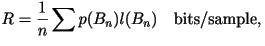 where where  is the length of the codeword for block .
- The higher the order, the lower the rate (better compression).
- The codes used in the above examples are Huffman
codes.
- We are only interested in lossless
data compression code. That is, given the code table and given the
compressed data, we should be able to rederive the original data. All of
the examples given above are lossless.
Theorem: Let  be the rate of an optimal n-th order lossless data compression
code (in bits/character). Then
be the rate of an optimal n-th order lossless data compression
code (in bits/character). Then
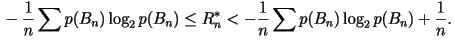
Since both upper and lower bounds of
approach the entropy rate, H, as n goes to infinity, we have
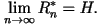 Thus, the theorem established that the
entropy rate is the rate of an optimal lossless data compression code. The
limit exists as long as the source is stationary. Thus, the theorem established that the
entropy rate is the rate of an optimal lossless data compression code. The
limit exists as long as the source is stationary.
V. Rate-Distortion Theory
Available at
Amazon.com
 | In lossy data compression, the
decompressed data need not be exactly the same as the original data.
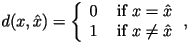
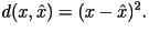
Often, it suffices to have a reasonably close approximation. A distortion measure is a mathematical entity which
specifies exactly how close the approximation is. Generally, it is a
function which assigns to any two letters  and
and  in the alphabet a
non-negative number denoted as in the alphabet a
non-negative number denoted as
 Here,
is the original data,
is the approximation, and Here,
is the original data,
is the approximation, and  is the amount of distortion between
and . The most common distortion measures are the Hamming distortion measure:
is the amount of distortion between
and . The most common distortion measures are the Hamming distortion measure:
 and the squared-error
distortion measure (which is only applicable when
is a set of numbers): and the squared-error
distortion measure (which is only applicable when
is a set of numbers):
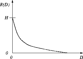
Rate-distortion theory says that for a given source and a given
distortion measure, there exists a function, R(D), called the
rate-distortion function. The typical shape of R(D) looks like
this:
If the source samples are independent of one another, the
rate-distortion function can be obtained by solving the constrained
minimization problem:
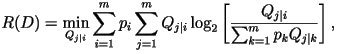 subject to the constraints that subject to the constraints that  and and
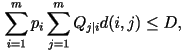 where where  is the distortion between the i-th and j-th letter in the
alphabet. Using Blahut's algorithm,
it may be possible to numerically calculate the rate-distortion function.
is the distortion between the i-th and j-th letter in the
alphabet. Using Blahut's algorithm,
it may be possible to numerically calculate the rate-distortion function.
Rate-distortion theory is based on the concept of block coding (similar
to above). A lossy block code is known as a vector
quantizer (VQ). The block length n of the code is known as
the VQ dimension.
Theorem: Assuming that the source is stationary and the
source samples are independent. For every  and for every
  , there exists a VQ of (sufficiently large) dimension
n with distortion no greater than , there exists a VQ of (sufficiently large) dimension
n with distortion no greater than
 and rate no more than and rate no more than
 Further more, there does not exist a VQ
with distortion Further more, there does not exist a VQ
with distortion  and rate less than
  . .
In essence, the theorem states
that R(D) is the rate-distortion performance of an optimal VQ. The
above theorem can be generalized to the case where the source is
stationary and ergodic.
VI. The Gap Between Theory and
Practice
- The theory holds when the block length n approaches infinity.
In real-time compression, the compression algorithm must wait for
n consecutive source samples before it can begin the compression.
When n is large, this wait (or delay) may be too long. For
example, in real-time speech compression, the speech signal is sampled
at 8000 samples/second. If n is say 4000, then the compression
delay is half a second. In a two-way conversation, this long delay may
not be desirable.
- The theory does not take into consideration the complexities
associated with the compression and decompression operations. Typically,
as the block length n increases, the complexities also increase.
Often, the rate of increase is exponential in n.
- The theory assumes that the statistical properties of the source is
known. In practice, this information may not be available.
- The theory assumes that there is no error in the compressed bit
stream. In practice, due to noise in the communication channel or
imperfection in the storage medium, there are errors in the compressed
bit stream.
All of these problems have been successfully solved
by researchers in the field.
VII. FAQs (Frequently Asked
Questions)
- What is
the difference between lossless and lossy compression?
- What
is the difference between compression rate and compression ratio?
- What is
the difference between ``data compression theory'' and ``source coding
theory''?
- What
does ``stationary'' mean?
- What does
``ergodic'' mean?
- What is the difference between lossless and lossy
compression?
In lossless data compression, the compressed-then-decompressed data
is an exact replication of the original data. On the other hand, in
lossy data compression, the decompressed data may be different from the
original data. Typically, there is some distortion between the original
and reproduced signal.
The popular WinZip program is an example of lossless compression.
JPEG is an example of lossy compression.
- What is the difference between compression rate and compression
ratio?
Historically, there are two main types of applications of data
compression: transmission and storage. An example of the former is
speech compression for real-time transmission over digital cellular
networks. An example of the latter is file compression (e.g.
Drivespace).
The term ``compression rate'' comes from the transmission camp, while
``compression ratio'' comes from the storage camp.
Compression rate is the rate of the compressed data (which we
imagined to be transmitted in ``real-time''). Typically, it is in units
of bits/sample, bits/character, bits/pixels, or bits/second. Compression
ratio is the ratio of the size or rate of the original data to the size
or rate of the compressed data. For example, if a gray-scale image is
originally represented by 8 bits/pixel (bpp) and it is compressed to 2
bpp, we say that the compression ratio is 4-to-1. Sometimes, it is said
that the compression ratio is 75%.
Compression rate is an absolute term, while compression ratio is a
relative term.
We note that there are current applications which can be considered
as both transmission and storage. For example, the above photograph of
Shannon is stored in JPEG format. This not only saves storage space on
the local disk, it also speeds up the delivery of the image over the
internet.
- What is the difference between ``data compression theory'' and
``source coding theory''?
There is no difference. They both mean the same thing. The term
``coding'' is a general term which could mean either ``data
compression'' or ``error control coding''.
- What does ``stationary'' mean?
Mathematically, a random process is stationary (or strict-sense
stationary) if for every positive integers
and  the vectors: the vectors:
 and and
 have the same probability distribution. have the same probability distribution.
We can think of ``stationarity'' in terms of our library example.
Suppose that we look at the first letter of all 100 million books and
see how often the first letter is `a', how often it is `b', and so on.
We will then get a probability distribution of the first letter of the
(random) book. If we repeat this experiment for the fifth and 105th
letters, we will get two other distributions. If all three distributions
are the same, we are inclined to believe that the book process is
stationary. To be sure, we should look at the joint distribution of the
first and second letters and compare it with the joint distribution of
the 101st and 102nd letters. If these two joint distributions are
roughly the same, we will be more convinced that the book process is
stationary.
In reality, the book process can not be stationary because the first
character can not be a SPACE.
- What does ``ergodic'' mean?
The strict mathematical definition of ergodicity is too complex to
explain. However, Shannon offered the following intuitive explanation:
``In an ergodic process every sequence produced by the process is the
same in statistical properties. Thus the letter frequencies, (the
pairwise) frequencies, etc., obtained from particular sequences, will,
as the lengths of the sequences increase, approach definite limits
independent of the particular sequence. Actually this is not true of
every sequence but the set for which it is false has probability zero.
Roughly the ergodic property means statistical homogeneity.''
VIII. References
- C. E. Shannon, A
Mathematical Theory of Communication (free pdf version)
- C. E. Shannon and W. Weaver, The
Mathematical Theory of Communication. ($13 paper version)
- C. E. Shannon, N. J. Sloane, and A. D. Wyner, Claude
Elwood Shannon: Collected Papers.
- C. E. Shannon, ``Prediction and Entropy of Printed English,"
available in Shannon:
Collected Papers.
- C. E. Shannon, ``Coding Theorems for a Discrete Source with a
Fidelity Criterion," available in Shannon:
Collected Papers.
- T. M. Cover and J. A. Thomas, Elements
of Information Theory.
- R. Gallager, Information
Theory and Reliable Communication.
- A. Gersho and R. M. Gray, Vector
Quantization and Signal Compression.
- K. Sayood, Introduction
to Data Compression.
- M. Nelson and J.-L. Gailly, The
Data Compression Book.
- A. Leon-Garcia, Probability
and Random Processes for Electrical Engineering. (Student
Solution Manual).
- A. Papoulis, Probability,
Random Variables, and Stochastic Processes.
- M. R. Schroeder, Computer
Speech: Recognition, Compression, Synthesis.
- G. Held and T. R. Marshall, Data
and Image Compression: Tools and Techniques.
- D. Hankerson, P. D. Johnson, and G. A. Harris, Introduction
to Information Theory and Data Compression .
Note: To anyone
interested in information theory, I can highly recommend two books:
Shannon's Collected
Papers and Cover and Thomas' Elements
of Information Theory. Collected
Papers includes a 1987 interview of Shannon by OMNI Magazine, almost
all of his papers on information theory and cryptography, his celebrated
Master's Theses on A Symbolic Analysis of Relay and Switching
Circuits, his Ph.D. dissertation on An Algebra for Theoretical
Genetics, his paper on the Scientific Aspects of Juggling, his
paper on A Mind Reading Machine, and much more. Elements
of Information Theory is now the standard textbook on information
theory. I have been using this textbook in my graduate-level information
theory course for the past seven years. I have had nothing but positive
feedback from students who have studied this book.
Nam Phamdo
Department of Electrical and Computer Engineering
State University of New York
Stony Brook, NY 11794-2350
phamdo@ieee.org
|