|
Grand Prismatic Spring, Yellowstone |
Environmental Geochemistry GEOL3150 |
|
Grand Prismatic Spring, Yellowstone |
Environmental Geochemistry GEOL3150 |
| Course Home | Syllabus | Schedule | Supplemental Materials | Links |
| Lecture PowerPoints (pdf) |
| Chapter 2 - Equilibrium Thermodynamics and Kinetics |
| Chapter 3 - Acid-Base Equilibria |
| Chapter 5 - Carbon Chemistry |
| Chapter 6 - Isotopes |
| Graphical Solutions for Problems | ||||
| Chapter 2 Problems | ||||
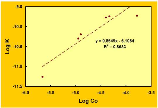
| Problem 2-38a. Plot of Log Co versus Log Rate. |
 |
|||
| Chapter 3 Problems | ||||
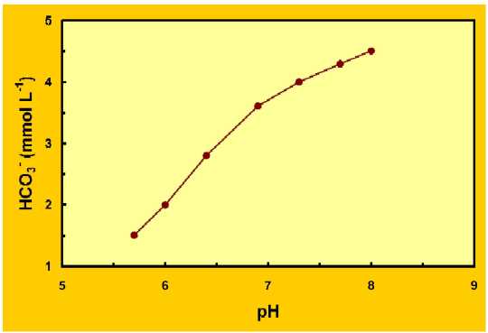
| Problem 3-28. Plot of bicarbonate ion concentration versus pH for the various water samples. |
 |
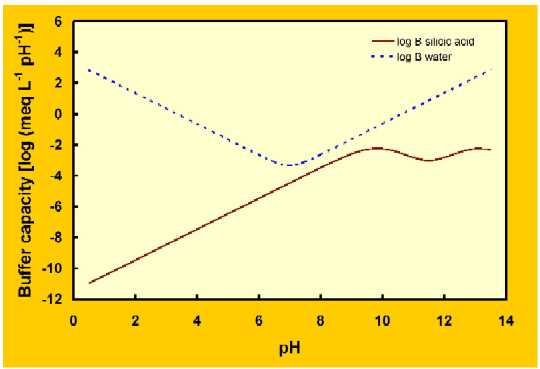
Problem 3-39. Plot of buffer capacity versus pH for 0.01 mol L-1 silicic acid solution. Only the first two dissociation steps are shown. |
|
|
| Chapter 4 Problems | ||||
| Template for Eh-pH diagrams. |
 |
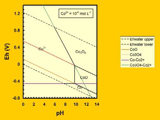
Problems 40-41. Eh-pH diagram for problems 40 and 41. Diagram drawn for [Co2+] = 10-6 mol L-1. Construction lines are shown on the diagram. |
|
|
| Chapter 5 Problems | ||||
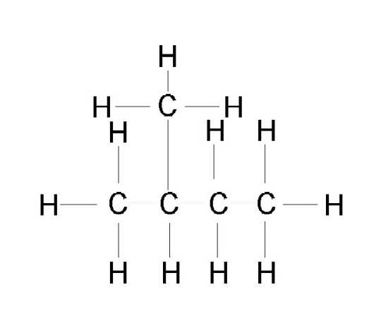
| Problem 5-39. Structural formula for 2-methylbutane. |
 |
Problem 5-41. Structural formula for 3-ethyl-2-methylpentane. | 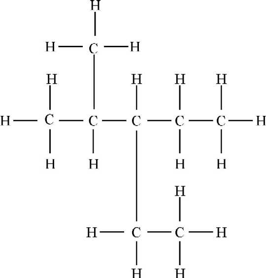 |
|
| Problem 5-42. Structural formula for 1,4-dimethylcyclohexane. | Problem 5-48. Structural formula for 1,2,3,6,9-pentachlorodibenzo-p-dioxin. | 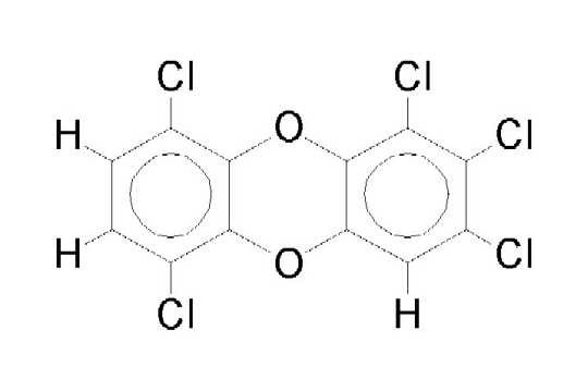 |
||
| Problem 5-52. Plot of C/N ratios versus d13C for various sediment samples from the Columbia river and continental margin. Two mixing lines are drawn, one between the reservoirs marine plankton and soil organic matter and the other between the reservoirs marine plankton and vascular plant material. Percent of these end members in each sample is estimated from these mixing lines. Note the marked correlation between sediment type and end member reservoirs. The end member reservoirs are taken from Figure 5-26 in the text. | 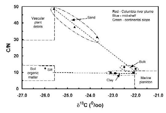 |
|||
| Chapter 6 Problems | ||||
| Problem 6-40. Plot of age of groundwater sample versus distance from the Danube river. | 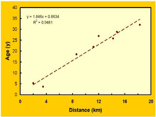 |
Problem 6-43. Plot of the natural log of the activity versus depth. The straight-line relationship indicates a constant sedimentation rate. | 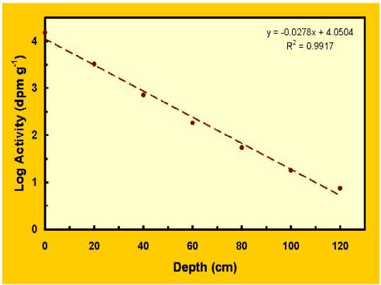 |
|
| Problem 6-44a. Plot of the natural log of the activity versus depth for Nainital lake. The straight-line relationship indicates a constant sedimentation rate. | 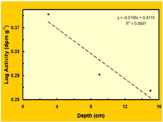 |
Problem 6-44b. Plot of the natural log of the activity versus depth for Sattal lake. The straight-line relationship indicates a constant sedimentation rate. | 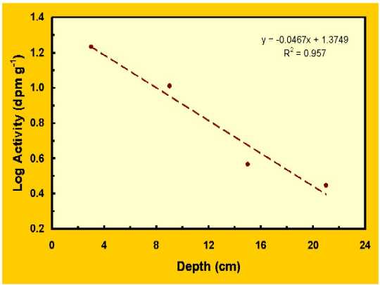 |
|
| Problem 6-54. Graphical solution for problem 6-54. G = groundwater, F = runoff from fields, R = runoff from feedlot, and W = contaminated well water. | 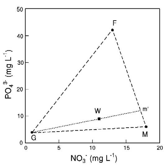 |
|||
| Chapter 7 Problems | ||||
| Problem 7-52a. Plot of Cads versus Csoln. | 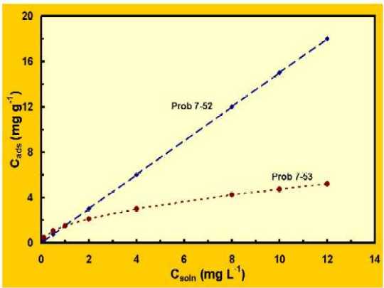 |
Problem 7-52b. Plot of log Cads versus log Csoln. The slope of the line gives the values for n and the y-intercept gives the value for K. | 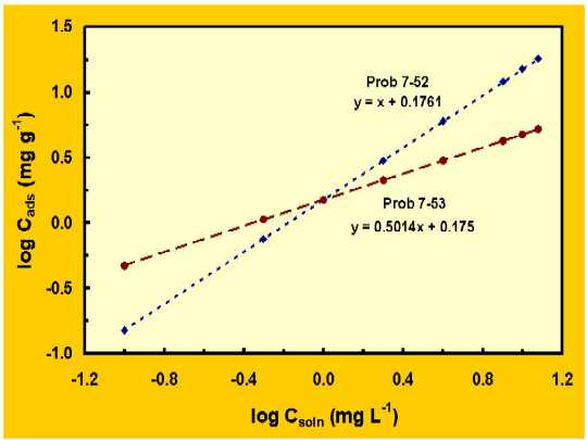 |
|
| Problem 7-54a. Plot of Cads versus Csoln. The shape of the curve, particularly the flattening of the curve at high concentrations, suggests that the data fit a Langmuir isotherm. | 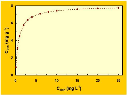 |
Problem 7-54b. Plot of 1/Cads versus 1/Csoln. The slope of the line = 1/KQo and the y-intercept = 1/Qo. | 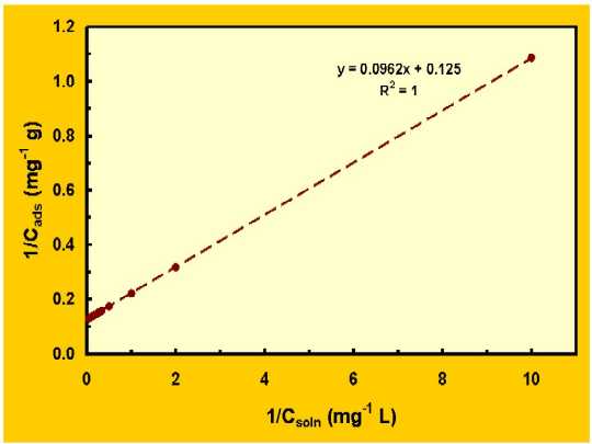 |
|
| Chapter 8 Problems | ||||
| Problem 8-88. Plot of 208Pb/206Pb versus 206Pb/207Pb for various sources and urban aerosols in Northwestern France. | 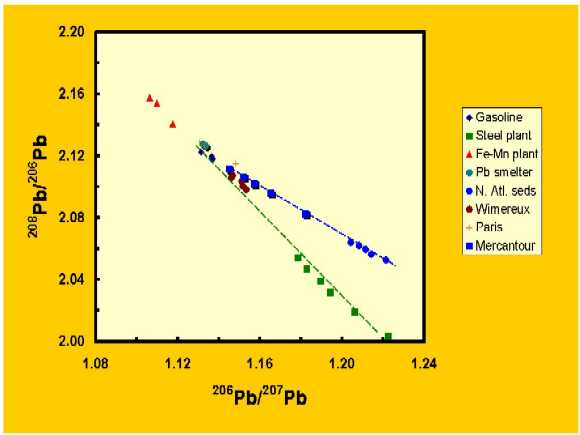 |
|||
| Problem 8-91a. Plot of enrichment factors, using bulk crust, for Zn and Pb versus age. | 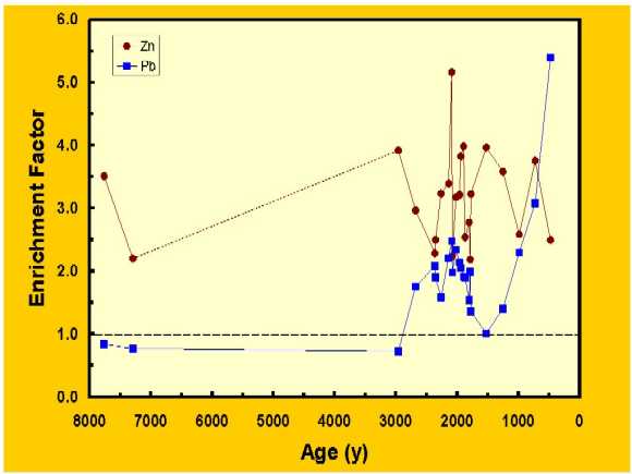 |
Problem 8-91b. Plot of enrichment factors, using upper crust, for Zn and Pb versus age. | 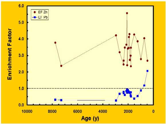 |
|
| Chapter 9 Problems | ||||
| Problem 9-77. Piper diagram for Colorado and Nile river waters. | 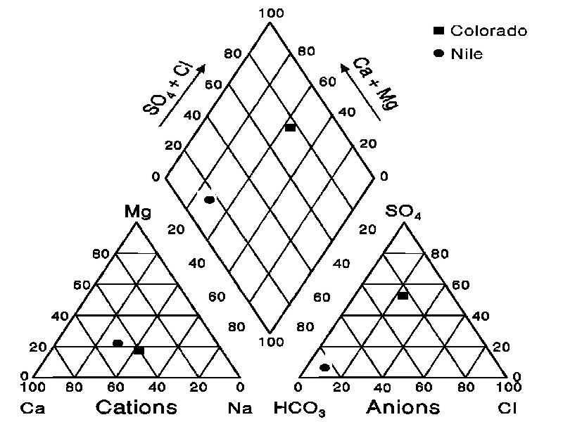 |
Problem 9-78. Piper diagram showing mixing between a tributary and a river. | 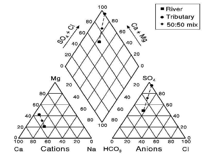 |
|
| Problem 9-106a. Plot of Cl/Br ratio versus distance of groundwater sample from the petrol station. The low Cl/Br ratios are indicative of groundwater samples contaminated by ethylene dibromide. The higher Cl/Br ratios are indicative of uncontaminated groundwater. | 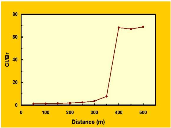 |
Problem 9-106b. Plot of Br- versus Cl-. The data form a linear array which suggests that the groundwater chemistry can be explained by simple mixing between uncontaminated groundwater and contaminated groundwater from the petrol station. | 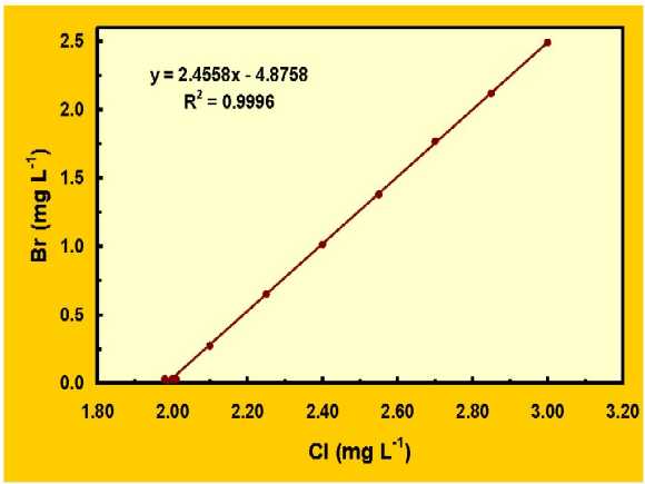 |
|