Back

Self Organized Polymer (SOP) model implemented on GPU (SOP-GPU)

SOP is a structure-based coarse-grained model of a polypeptide chain, which described the time-evolution of the chain by following the Langevin dynamics in three dimensions. The model uses a simple and computationally light yet accurate force field in terms of describing the macroscopic physical properties of a biomolecular system. Previous studies have shown that the SOP model describes well the mechanical properties of proteins, including the Green Fluorescent Protein [1], the tubulin dimer [2] and kinesin [3]. The SOP-model has also been employed to explore the kinetics and to map the free energy landscape of various biomolecules such as the tetrahymena ribozyme [4], riboswitch aptamers [5], GroEL [6], DHFR [7] protein kinase A [8] and myosin V [9]. In the SOP model, each amino acid residue of a chain is representated by just one C_α-particle. In addition, Langevin simulations are accelerated on a GPU ~10-200-fold, depending on size of the system in question. A combination of these factors enables one to follow the system dynamics on a very long centisecond to second timescale. This is a range of experimental timescales in the Atomic Force Microscopy (AFM) and optical tweezer-based dynamic force measurements on single proteins, multimeric proteins and protein tandems, protein-protein complexes and aggregates, protein fibers, and protein assemblies. Currently, it remains virtually impossible to reach the biologically relevant millisecond to second timescales even for a very small system of a few tens of residues using conventional all-atom Molecular Dynamics (MD) methods in explicit and implicit solvent (water) implemented on the most powerful distributed computer clusters. In the context of dynamic force measurements in silico, force-loading conditions used in all-atom MD simulation approaches (the force-loading rates and cantilever tip geometry), are different from those employed in the experimental dynamic force microscopy. In this regard, the SOP-GPU model incorporated into the SOP-GPU package is the only known approach, which enables researchers to explore the mechano-chemical properties of biological systems

• in the experimental subsecond timescale


• using realistic conditions of force application

This is farely important, rendering the fact that the kinetics (pathways, intermediate states), thermodynamics (transition barriers and working distances), and mechanisms all change with the rate r_f of a force load f_ext=r_ft (force-ramp), and with the force level f_ext=const (force-clamp). When the X-ray structure of a biological system is known (from Protein Data Bank or other depositories), the SOP-GPU model enables researchers to explore

• force-induced elongation, conformational transitions, and unfolding in proteins, RNA and DNA


• mechanically driven dissociation of biomolecular complexes and aggregates


• forced indentation of protein fibers and capsids of animal and plant viruses

This can be readily achieved in reasonable wall-clock time using the SOP-GPU package. Hence, the results of single molecule experiments and simulations can be compared directly, which helps researchers provide meaningful interpretation of the results of experimental force measurements, i.e. dynamic signatures in the force spectra and force-indentation curves.

In the SOP model [1,4,10], each residue is described using a single interaction center (C_α-atom). The dynamics of the i-th C_α-particle are obtained by following the Langevin equations in the overdamped limit:

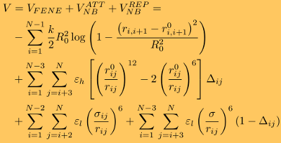
where ξ is the friction coefficient, and f(R_i)=−∂V/∂R_i is the molecular force exerted on the i-th particle due to the potential energy V. Here, G_i(t) is the Gaussian distributed random force with zero mean and delta function correlations (white noise). The random force takes into consideration the stochastic collisions of protein residues with the solvent (water) molecules. The potential energy function of a protein conformation V (force field), specified in terms of the coordinates of the C_α-particles, {R} = R₁, R₂, ... R_n , is given by

where the distance between any two interacting residues i and i+1 is r_i,i+1, whereas r⁰_i,i+1 is its value in the native (PDB) structure. The first term in the equation is the finite extensible nonlinear elastic (FENE) potential, which describes the backbone chain connectivity. Here, R₀=2 Å is the tolerance in the change of a covalent bond, and k=1.4 N/m is the force constant. The second term in the equation is the Lennard-Jones potential (V_NB^ATT), which accounts for the native interactions that stabilize the (native) folded state. In the SOP model, it is assumed that when the non-covalently linked residues i and j (|i - j| > 2) are within the cutoff distance R_C in the native state, i.e., r_ij < R_C, then Δ_ij=1, and zero otherwise. The value of ε_h specifies the strength of the nonbonded interactions. The typical values of ε_h are in the 1.0-1.5 kcal/mol range, depending on the secondary structure element in question. All non-native interactions (fourth term in the above equation) are treated as repulsive (V_NB^REP). Additional constraint are imposed on the bond angle formed by residues i, i+1, and i+2 by including the repulsive potential with parameters ε_l=1 kcal/mol and σ=3.8 Å, which quantify, respectively, the strength and the range of repulsion. To ensure self-avoidance of the protein chain, the σ value is set to σ=3.8 Å.

Because GPUs differ from CPUs in several fundamental ways, the CPU-based methods for biomolecular simulations cannot be easily translated nor simply adapted to a GPU. In molecular simulations, the particle-particle interactions are described by the same empirical potential energy function (force field), and the system dynamics is obtained by solving numerically the same equations of motion for all particles. For the SOP model, we have developed the numerical procedures for generation of Verlet lists and random forces, for the computation of forces due to covalent and non-covalent interactions, and for the numerical integration of Langevin equations of motion [10]. A detailed description of the numerical algorithms can be found in our recent paper here.

On a GPU, there are two main optimization strategies that allow to compute forces due to binary (particle-particle) interactions. In the first approach, all forces acting on one particle are computed in one thread, which requires running N threads to obtain the force values for all particles. We refer to this procedure as the particle based parallelization approach. The use of this approach requires the computation of the same force increment df, acting on the i-th and j-th particles, twice in the i-th and j-th computational threads. To describe the long-range interactions, we use a general notion that long-range interactions vanish over some characteristic distance. This allows us to generate and use Verlet lists. Using the particle based parallelization approach, Verlet lists can be easily re-generated on a GPU device to accelerate the computation of the potential energy terms. In the interacting pair based parallelization approach, force calculations are performed for all (i,j)-pairs using a total of P independent threads of computations, which is equal the number of pairs of interacting particles. Then, 2P force values are saved to different locations in the GPU global memory. In the interacting pair based parallelization approach, generating a Verlet list amounts to forming a vector of all pairs of coupled residues for one potential energy term. To obtain an ordered Verlet list, the list has to be sorted or updated on a CPU. It is more efficient to compute interparticle distances on a GPU, copy them to the CPU DRAM, and then generate a new list (see Ref.[10] for more detail).

The Langevin equations of motion for each residue (C_α-particle) are integrated numerically using the first order integration scheme (Ermak-McCammon algorithm) [10],

where h is the integration timestep. Benchmark tests of the accuracy of numerical integration, which assess the magnitude of numerical error accumulated over many billions of iterations, show that in long simulations on a GPU device single precision arithmetic and the Ermak-McCammon algorithm can be used to describe accurately the mechanical properties of biomolecules.

Langevin simulations require a reliable source of normally distributed (pseudo)-random numbers, g_i,α (α = x, y, and z, and = 1,2,...,n), to compute the three components of the Gaussian random force

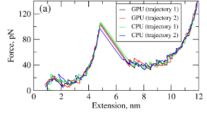
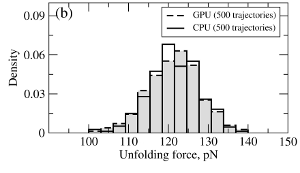
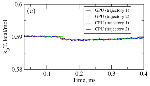
where T is the absolute temperature (k_b is the Boltzmann's constant). A (pseudo)-random number generator (RNG) produces a sequence of random numbers u_i,α,a uniformly distributed in the unit interval [0,1], which is then translated into a sequence of normally distributed random numbers with zero mean and unit variance (g_i,α) using variety of methods. In the SOP-GPU package we utilize the well-known Box-Mueller transformation. A detailed description of the numerical algorithms for the implementation of random number generators (RNGs) on the GPU device is given here.

We have tested the performance of the SOP-GPU package (written in CUDA - a dialect of C and C++ programming languages) on a NVIDIA GPU Tesla C1060 (MIPT), and have compared the results against the performance of the optimized C code (SOP program) on a dual Quad Core Xeon 2.83 GHz of a similar level of technology. We have analyzed the results of CPU- and GPU-based computations by comparing the force spectra, i.e. f versus X force-extension profiles, the distributions of unfolding forces (peak forces in the force spectra), and the average temperature ⟨T⟩, for the all-β sheet WW-domain (see Figure 1). Aside from small deviations due to the different initial conditions, the profiles of f(X) and ⟨T⟩, and the unfolding force histograms, obtained on the CPU and on the GPU, agree very well.

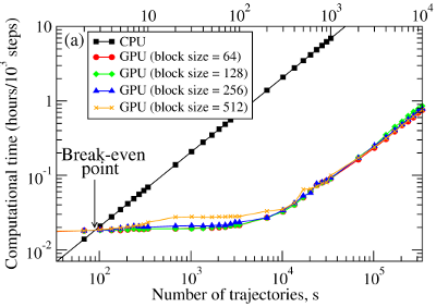
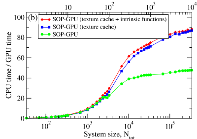
We have compared the overall performance of an end-to-end application of the SOP-GPU program with the heavily tuned CPU-based implementation (SOP program) in describing the Langevin dynamics of the WW domain at equilibrium. We profiled the computational performance of the SOP-GPU program as a function of the number of independent trajectories s running concurrently on the GPU (many-runs-per-GPU approach). While the single CPU core generates one trajectory at a time, the GPU device is capable of running many trajectories at the same time. The results (see Figure 2a) show that, for the WW domain (N = 34), the GPU accelerates computations starting from 3 independent runs, which is equivalent to a single run for a system of N≈102 residues (one-run-per-GPU approach). This is the so-called break-even point. While the simulation time on the CPU scales linearly with s (or with N), the scaling on the GPU in this regime is sublinear (nearly constant) up to N≈10⁴ (s≈300 for the WW domain). At this point, the GPU shows significant performance gains relative to the CPU reaching the maximum 80–90-fold speedup (see Figure 2b). The amount of GPU on-board memory, i.e. ~4 GB (Tesla C1060), is sufficient to describe long Langevin dynamics for large biomolecular systems of ~10⁴ residues, i.e., comparable in size with the fibrinogen dimer (Fb)₂.