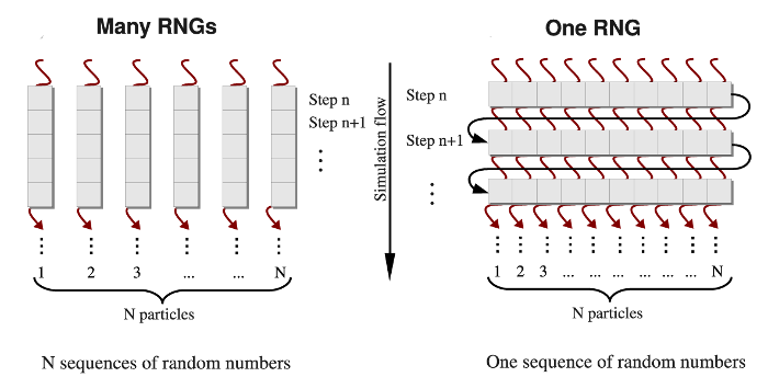
Back

Generation of pseudo-random numbers on graphics processors

Pseudo-random number generators are used in many computer applications such as simulations of stochastic systems, numerical analysis, probabilistic algorithms, etc. Numerical modeling of biological systems and processes, e.g., all-atom MD simulations in implicit solvent [1, 2], Langevin simulations [14], and Monte Carlo simulations [4], all require generation of a large number of independent random variables at each step of a simulation run. We developed two approaches for implementation of random number generators (RNGs) on a graphics processing unit (GPU). In the one-RNG-per-thread approach, one RNG produces a stream of random numbers in each thread of execution, whereas the one-RNG-for-all-threads method builds on the ability of different threads to communicate, thus, sharing random seeds across an entire GPU device. An RNG produces a sequence of random numbers, u_i, which is supposed to imitate independent and uniformly distributed random variates from the unit interval (0,1). There are three main requirements for a numerical implementation of an RNG: (1) good statistical properties, (2) high computational speed, and (3) low memory usage. Because a deterministic sequence of random numbers comes eventually to a starting point, u_n+p =u_n, an RNG should also have a long period p [3]. In addition, an RNG must pass rigorous statistical tests of randomness (i.e., for independence and for uniformity), and some application-based tests of randomness that offer exact solutions to the test applications [3, 8-10]. Indeed, using random numbers of poor statistical quality might result in insufficient sampling, unphysical correlations, and even unrealistic results, which might lead to errors in practical applications. We developed the GPU-based realizations of several RNGs, which provide pseudo-random numbers of high statistical quality, using the cycle division paradigm [13].

Different methods are used to generate the Gaussian distributed random variates g_i from the uniformly distributed random numbers u_i (i=1,2,...,n) [5-7]. Here, we adopt the most commonly used Box-Mueller transformation [7]. In the one-RNG-per-thread approach, the basic idea is to partition a single sequence of random numbers among many computational threads running concurrently across an entire GPU device, each producing a stream of random numbers. Since most RNG algorithms, including LCG, Ran2, and Hybrid Taus, are based on sequential transformations of the current state [4], then the most common way of partitioning the sequence is to provide each thread with different seeds while also separating the threads along the sequence so as to avoid possible inter-stream correlations (see Figure 1, left panel). On the other hand, several generators, including the Mersenne Twister and Lagged Fibonacci algorithms, which employ recursive transformations, allow one to leap ahead in a sequence of random variates and to produce the (n + 1)-st random number without knowing the previous, n-th number [12]. The leap size, which, in general, depends on a choice of parameters for an RNG, can be properly adjusted to the number of threads (number of particles N), or multiples of N (M×N). Then, all N random numbers can be obtained simultaneously, i.e. the j-th thread produces numbers j, j+N, j+2N,..., etc. (j=1,2,...,n). At the end of each simulation step, threads of execition must be syncronized to update the current RNG state. Hence, the same RNG state can be shared by all threads, each updating just one elements of the state. We refer to this as the one-RNG-for-all-threads approach (Figure 1, right panel).

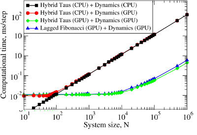
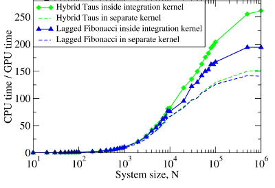
We employed these methods to develop GPU-based implementations of the Linear Congruent Generator (LCG) [4], and the Ran2 [4], Hybrid Taus [4, 11], and additive Lagged Fibonacci algoritms [4, 12]. These generators have been incorporated into the program for Langevin simulations of biomolecules fully implemented on the GPU. The ∼250-fold computational speedup, attained on the GPU device, allows us to carry out molecular simulations in a stochastic thermostat. Using this speedup we are now capable of performing, e.g., single-molecule dynamic force measurements in silico to explore the mechanical properties of large-size supramolecular biological assemblies, such as the fibrinogen oligomer (Fb)₂ and bacteriophage HK97, in the experimental subsecond timescale using realistic force-loads.

We tested RNGs implemented on a GPU in Langevin simulations of N Brownian oscillators using the Hybrid Taus and additive Lagged Fibonacci algorithms. We compared the computational time as a function of the system size N for three different implementations of Langevin simulations:

• random numbers and Langevin Dynamics are generated on a CPU


• random numbers, obtained on the CPU, are transfered to the GPU and used to generate Langevin Dynamics on the GPU


• random numbers and Langevin Dynamics are generated on the GPU

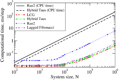
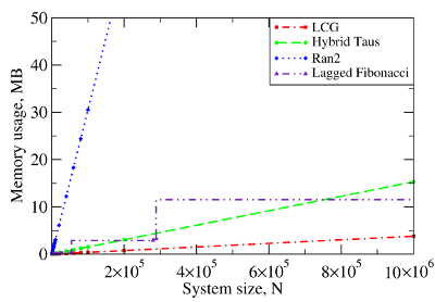
We also benchmarked the computational efficiency of the GPU-based realizations of the Ran2, Hybrid Taus, and Lagged Fibonacci algorithms using Langevin simulations of N Brownian oscillators in three dimensions. For each system size N, we ran one trajectory for 10⁶ simulation steps. All N threads were synchronized at the end of each step to emulate an LD simulation run of a biomolecule on a GPU. The associated execution time and memory usage are profiled in Figure 3 below.

We find that on a GPU Ran2 is the most demanding generator as compared to the Hybrid Taus, and Lagged Fibonacci RNGs (Figure 3, left panel). Using Ran2 in Langevin simulations to obtain a single trajectory over 10⁹ steps for a system of N=10⁴ particles requires additional ∼264 hours of wall-clock time. The associated memory demand for Ran2 RNG is quite high, i.e. >250MB for N=10⁶ (Figure 3, right panel). Because in biomolecular simulations a large memory area is needed to store parameters of the force field, Verlet lists, interparticle distances, etc., the high memory demand might prevent one from using Ran2 in the simulations of a large system. Also, implementing the Ran2 RNG in Langevin simulations on the GPU does not lead to a substantial speedup (Figure 3, left panel). By contrast, the Hybrid Taus and Lagged Fibonacci RNGs are both light and fast in terms of the memory usage and the execution time (Figure 3). These generators require a small amount of memory, i.e. <15−20MB, even for a large system of as many as N=10⁶ particles.