An ordered rooted tree is a rooted tree whose subtrees are put into a definite order and are, themselves, ordered rooted trees. An empty tree and a single vertex with no descendants (no subtrees) are ordered rooted trees.
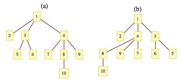
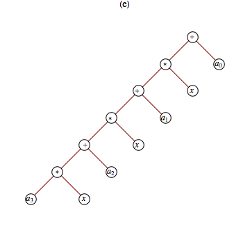
The trees in Figure 10.4.2 are identical rooted trees, with root 1, but as ordered trees, they are different.
Figure10.4.2.Two different ordered rooted trees
If a tree rooted at \(v\) has \(p\) subtrees, we would refer to them as the first, second,..., \(p^{th}\) subtrees. There is a subtle difference between certain ordered trees and binary trees, which we define next.
Definition10.4.3.Binary Tree.
A tree consisting of no vertices (the empty tree) is a binary tree
A vertex together with two subtrees that are both binary trees is a binary tree. The subtrees are called the left and right subtrees of the binary tree.
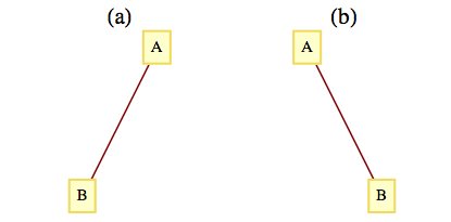
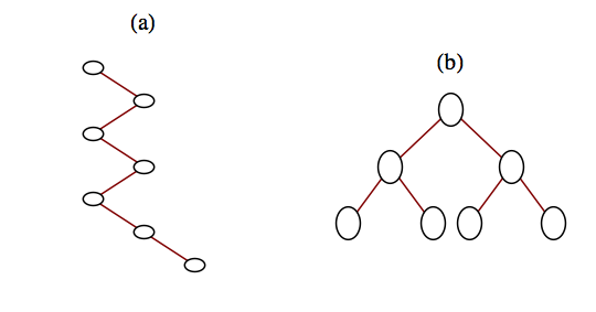
The difference between binary trees and ordered trees is that every vertex of a binary tree has exactly two subtrees (one or both of which may be empty), while a vertex of an ordered tree may have any number of subtrees. But there is another significant difference between the two types of structures. The two trees in Figure 10.4.4 would be considered identical as ordered trees. However, they are different binary trees. Tree (a) has an empty right subtree and Tree (b) has an empty left subtree.
Figure10.4.4.Two different binary treesList10.4.5.Terminology and General Facts about Binary Trees
A vertex of a binary tree with two empty subtrees is called a leaf. All other vertices are called internal vertices.
The number of leaves in a binary tree can vary from one up to roughly half the number of vertices in the tree (see Exercise 4 of this section).
The maximum number of vertices at level \(k\) of a binary tree is \(2^k\) , \(k\geq 0\) (see Exercise 6 of this section).
A full binary tree is a tree for which each vertex has either zero or two empty subtrees. In other words, each vertex has either two or zero children. See Exercise 10.4.6.7 of this section for a general fact about full binary trees.
Subsection10.4.2Traversals of Binary Trees
The traversal of a binary tree consists of visiting each vertex of the tree in some prescribed order. Unlike graph traversals, the consecutive vertices that are visited are not always connected with an edge. The most common binary tree traversals are differentiated by the order in which the root and its subtrees are visited. The three traversals are best described recursively and are:
Preorder Traversal:
Visit the root of the tree.
Preorder traverse the left subtree.
Preorder traverse the right subtree.
Inorder Traversal:
Inorder traverse the left subtree.
Visit the root of the tree.
Inorder traverse the right subtree.
Postorder Traversal:
Postorder traverse the left subtree.
Postorder traverse the right subtree.
Visit the root of the tree.
Any traversal of an empty tree consists of doing nothing.
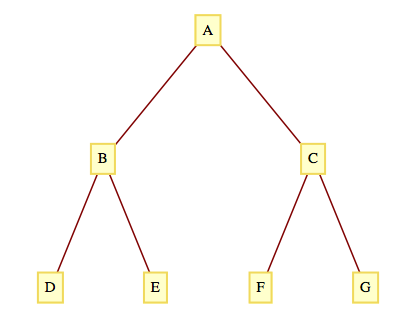
For the tree in Figure 10.4.7, the orders in which the vertices are visited are:
A-B-D-E-C-F-G, for the preorder traversal.
D-B-E-A-F-C-G, for the inorder traversal.
D-E-B-F-G-C-A, for the postorder traversal.
Figure10.4.7.A Complete Binary Tree to Level 2
Binary Tree Sort. Given a collection of integers (or other objects than can be ordered), one technique for sorting is a binary tree sort. If the integers are \(a_1\text{,}\)\(a_2, \ldots \text{,}\)\(a_n\text{,}\)\(n\geq 1\text{,}\) we first execute the following algorithm that creates a binary tree:
Algorithm10.4.8.Binary Sort Tree Creation.
Insert \(a_1\) into the root of the tree.
For k := 2 to n // insert \(a_k\) into the tree
r = \(a_1\)
inserted = false
while not(inserted):
\(\quad \)if \(a_k < r\text{:}\)
\(\quad \quad \quad \)if \(r\) has a left child:
\(\quad \quad \quad \quad\)r = left child of \(r\)
\(\quad \quad \quad\) else:
\(\quad \quad \quad \quad\)make \(a_k\) the left child of \(r\)
\(\quad \quad \quad \quad\)inserted = true
\(\quad \quad\)else:
\(\quad \quad \quad \)if \(r\) has a right child:
\(\quad \quad \quad \quad\)r = right child of \(r\)
\(\quad \quad \quad\) else:
\(\quad \quad \quad \quad\)make \(a_k\) the right child of \(r\)
\(\quad \quad \quad \quad\)inserted = true
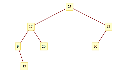
If the integers to be sorted are 25, 17, 9, 20, 33, 13, and 30, then the tree that is created is the one in Figure 10.4.9. The inorder traversal of this tree is 9, 13, 17, 20, 25, 30, 33, the integers in ascending order. In general, the inorder traversal of the tree that is constructed in the algorithm above will produce a sorted list. The preorder and postorder traversals of the tree have no meaning here.
Figure10.4.9.A Binary Sorting Tree
Subsection10.4.3Expression Trees
A convenient way to visualize an algebraic expression is by its expression tree. Consider the expression
\begin{equation*}
X = a*b - c/d + e.
\end{equation*}
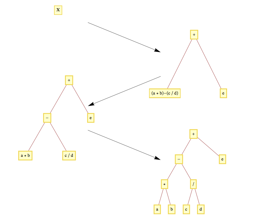
Since it is customary to put a precedence on multiplication/divisions, \(X\) is evaluated as \(((a*b) -(c/d)) + e\text{.}\) Consecutive multiplication/divisions or addition/subtractions are evaluated from left to right. We can analyze \(X\) further by noting that it is the sum of two simpler expressions \((a*b) - (c/d)\) and \(e\text{.}\) The first of these expressions can be broken down further into the difference of the expressions \(a*b\) and \(c/d\text{.}\) When we decompose any expression into \((\textrm{left expression})\textrm{operation} (\textrm{right expression})\text{,}\) the expression tree of that expression is the binary tree whose root contains the operation and whose left and right subtrees are the trees of the left and right expressions, respectively. Additionally, a simple variable or a number has an expression tree that is a single vertex containing the variable or number. The evolution of the expression tree for expression \(X\) appears in Figure 10.4.10.
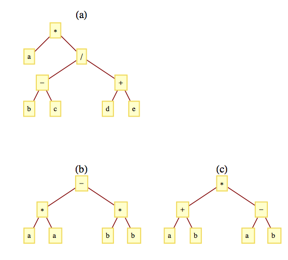
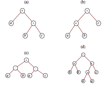
If we intend to apply the addition and subtraction operations in \(X\) first, we would parenthesize the expression to \(a*(b - c)/(d + e)\text{.}\) Its expression tree appears in Figure 10.4.12(a).
The expression trees for \(a^2-b^2\) and for \((a + b)*(a - b)\) appear in Figure 10.4.12(b) and Figure 10.4.12(c).
Figure10.4.12.Expression Tree Examples
The three traversals of an operation tree are all significant. A binary operation applied to a pair of numbers can be written in three ways. One is the familiar infix form, such as \(a + b\) for the sum of \(a\) and \(b\text{.}\) Another form is prefix, in which the same sum is written \(+a b\text{.}\) The final form is postfix, in which the sum is written \(a b+\text{.}\) Algebraic expressions involving the four standard arithmetic operations \((+,-,*, \text{and}
/)\) in prefix and postfix form are defined as follows:
List10.4.13.Prefix and postfix forms of an algebraic expression
Prefix
A variable or number is a prefix expression
Any operation followed by a pair of prefix expressions is a prefix expression.
Postfix
A variable or number is a postfix expression
Any pair of postfix expressions followed by an operation is a postfix expression.
The connection between traversals of an expression tree and these forms is simple:
The preorder traversal of an expression tree will result in the prefix form of the expression.
The postorder traversal of an expression tree will result in the postfix form of the expression.
The inorder traversal of an operation tree will not, in general, yield the proper infix form of the expression. If an expression requires parentheses in infix form, an inorder traversal of its expression tree has the effect of removing the parentheses.
The preorder traversal of the tree in Figure 10.4.10 is \(+-*ab/cd e\text{,}\) which is the prefix version of expression \(X\text{.}\) The postorder traversal is \(ab*cd/-e+\text{.}\) Note that since the original form of \(X\) needed no parentheses, the inorder traversal, \(a*b-c/d+e\text{,}\) is the correct infix version.
Subsection10.4.4Counting Binary Trees
We close this section with a formula for the number of different binary trees with \(n\) vertices. The formula is derived using generating functions. Although the complete details are beyond the scope of this text, we will supply an overview of the derivation in order to illustrate how generating functions are used in advanced combinatorics.
Let \(B(n)\) be the number of different binary trees of size \(n\) (\(n\) vertices), \(n \geq 0\text{.}\) By our definition of a binary tree, \(B(0) = 1\text{.}\) Now consider any positive integer \(n + 1\text{,}\)\(n \geq 0\text{.}\) A binary tree of size \(n + 1\) has two subtrees, the sizes of which add up to \(n\text{.}\) The possibilities can be broken down into \(n + 1\) cases:
Case 0: Left subtree has size 0; right subtree has size \(n\text{.}\)
Case 1: Left subtree has size 1; right subtree has size \(n - 1\text{.}\)
\(\quad \quad \)\(\vdots\)
Case \(k\text{:}\) Left subtree has size \(k\text{;}\) right subtree has size \(n - k\text{.}\)
\(\quad \quad \)\(\vdots\)
Case \(n\text{:}\) Left subtree has size \(n\text{;}\) right subtree has size 0.
In the general Case \(k\text{,}\) we can count the number of possibilities by multiplying the number of ways that the left subtree can be filled, \(B(k)\text{,}\) by the number of ways that the right subtree can be filled. \(B(n-k)\text{.}\) Since the sum of these products equals \(B(n + 1)\text{,}\) we obtain the recurrence relation for \(n\geq 0\text{:}\)
The coefficients after the first one are all negative and there is a singularity at 0 because of the \(\frac{1}{z}\) term. However if we do the same with \(G_2\) we get
This sequence of numbers is often called the Catalan numbers. For more information on the Catalan numbers, see the entry A000108 in The On-Line Encyclopedia of Integer Sequences 1 .
Subsection10.4.5SageMath Note - Power Series
It may be of interest to note how the extended power series expansions of \(G_1\) and \(G_2\) are determined using Sage. In Sage, one has the capability of being very specific about how algebraic expressions should be interpreted by specifying the underlying ring. This can make working with various algebraic expressions a bit more confusing to the beginner. Here is how to get a Laurent expansion for \(G_1\) above.
The first Sage expression above declares a structure called a ring that contains power series. We are not using that whole structure, just a specific element, G1. So the important thing about this first input is that it establishes z as being a variable associated with power series over the integers. When the second expression defines the value of G1 in terms of z, it is automatically converted to a power series.
The expansion of \(G_2\) uses identical code, and its coefficients are the values of \(B(n)\text{.}\)
In Chapter 16 we will introduce rings and will be able to take further advantage of Sage’s capabilities in this area.
Exercises10.4.6Exercises
1.
Draw the expression trees for the following expressions:
\(\displaystyle a(b + c)\)
\(\displaystyle a b + c\)
\(\displaystyle a b + a c\)
\(\displaystyle b b - 4 a c\)
\(\displaystyle \left(\left(a_3 x + a_2\right)x +a_1\right)x + a_0\)
\begin{equation*}
\begin{array}{cccc}
& \text{Preorder} & \text{Inorder} & \text{Postorder} \\
(a) & \cdot a + b c & a\cdot b+c & a b c + \cdot \\
(b) & +\cdot a b c & a\cdot b+c & a b\cdot c+ \\
(c) & +\cdot a b\cdot a c & a\cdot b+a\cdot c & a b\cdot a c\cdot + \\
\end{array}
\end{equation*}
4.
Verify the formula for \(B(n)\text{,}\)\(0 \leq n \leq 3\) by drawing all binary trees with three or fewer vertices.
5.
Draw a binary tree with seven vertices and only one leaf. Your answer won’t be unique. How many different possible answers are there?
Draw a binary tree with seven vertices and as many leaves as possible.
There are \(2^6=64\) different possible answers to part (a). The answer to (b) is unique.
Figure10.4.17.
6.
Prove that the maximum number of vertices at level \(k\) of a binary tree is \(2^k\) and that a tree with that many vertices at level \(k\) must have \(2^{k+1}-1\) vertices.
7.
Prove that if \(T\) is a full binary tree, then the number of leaves of \(T\) is one more than the number of internal vertices (non-leaves).
Basis: A binary tree consisting of a single vertex, which is a leaf, satisfies the equation \(\text{leaves} = \textrm{internal vertices} + 1\)
Induction:Assume that for some \(k\geq 1\text{,}\) all full binary trees with \(k\) or fewer vertices have one more leaf than internal vertices. Now consider any full binary tree with \(k+1\) vertices. Let \(T_A\) and \(T_B\) be the left and right subtrees of the tree which, by the definition of a full binary tree, must both be full. If \(i_A\) and \(i_B\) are the numbers of internal vertices in \(T_A\) and \(T_B\text{,}\) and \(j_A\) and \(j_B\) are the numbers of leaves, then \(j_A=i_A+1 \) and \(j_B=i_B+1\text{.}\) Therefore, in the whole tree,
\begin{equation*}
\begin{split}
\textrm{the number of leaves} & =j_A+j_B\\
&=\left(i_A+1\right)+\left(i_B+1\right)\\
&=\left(i_A+i_B+1\right)+1\\
&=(\textrm{number of internal vertices})+1
\end{split}
\end{equation*}
Solution 2:
Imagine building a full binary tree starting with a single vertex. By continuing to add leaves in pairs so that the tree stays full, we can build any full binary tree. Our starting tree satisfies the condition that the number of leaves is one more than the number of internal vertices . By adding a pair of leaves to a full binary tree, an old leaf becomes an internal vertex, increasing the number of internal vertices by one. Although we lose a leaf, the two added leaves create a net increase of one leaf. Therefore, the desired equality is maintained.
8.
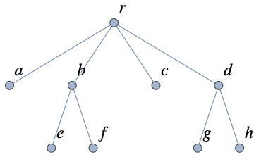
There is a one to one correspondence between ordered rooted trees and binary trees. If you start with an ordered rooted tree, \(T\text{,}\) you can build a binary tree \(B\) with an empty right subtree by placing the the root of \(T\) at the root of \(B\text{.}\) Then for every vertex \(v\) from \(T\) that has been placed in \(B\text{,}\) place it’s leftmost child (if there is one) as \(v\)’s left child in \(B\text{.}\) Make \(v\)’s next sibling (if there is one) in \(T\) the right child in \(B\text{.}\)
Figure10.4.18.An ordered rooted tree with root \(r\text{.}\)
Figure10.4.19.Blue (left) and Red (right) links added to the ordered rooted tree with root r.
Figure10.4.20.Binary tree corresponding to the ordered rooted tree.
Why will \(B\) have no right children in this correspondence?
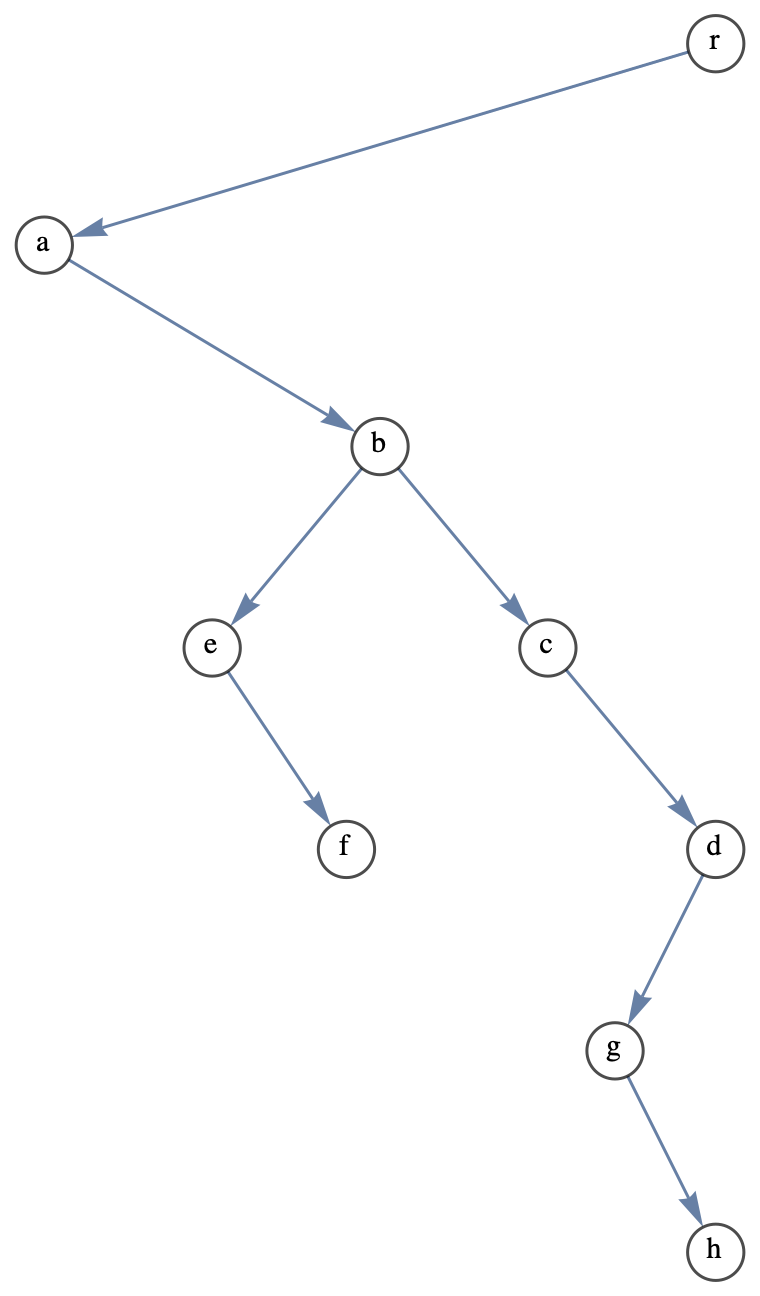
Draw the binary tree that is produced by the ordered rooted tree in Figure 10.4.21.
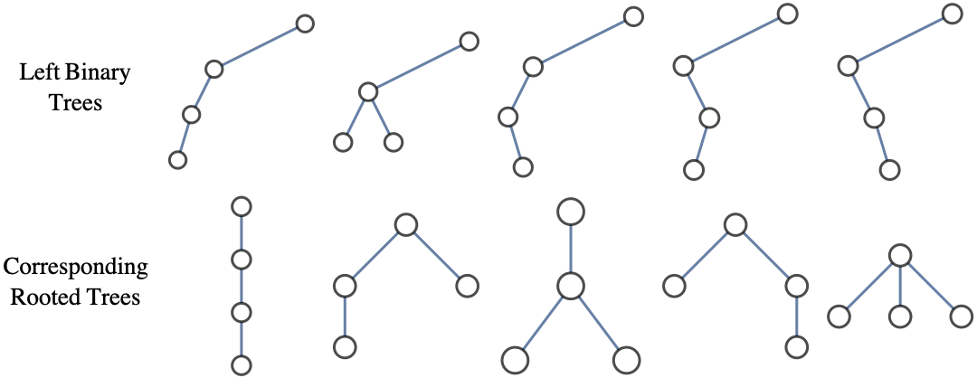
The left subtree of the binary tree in Figure 10.4.22 is one of 5 different binary trees with three vertices. Draw each of them and also the ordered rooted tree that each corresponds with.
What does this correspondence tell us about how the numbers of different binary trees and ordered rooted trees are related?
Figure10.4.21.What binary tree does this correspond with?
Figure10.4.22.What ordered rooted tree does this correspond with?
The root of \(B\) is the root of the corresponding ordered rooted tree, which as no siblings.
Figure10.4.23.
Figure10.4.24.
The number of ordered rooted trees with \(n\) vertices is equal to the number of binary trees with \(n-1\) vertices, \(\frac{1}{n} \binom{2(n-1)}{n-1}\)

![An ordered rooted tree with root \(r\) specifed by the dictionary of children {r:[a,d,c],a:[b,c],e:[f,g,h]}.](images/fig-ex-ordered-tree.png)
![An ordered rooted tree with root r specifed by the dictionary of children {r:[a,d,c],a:[b,c],e:[f,g,h]} with colored edges added to indicate the correspondence with a binary tree.](images/fig-ex-ordered-tree-linked.png)
![The binary tree corresponding with the ordered rooted tree rooted at r specified by the dictionary of children {r:[a,d,c],a:[b,c],e:[f,g,h]}.](images/fig-ex-binary-tree.png)
![A binary tree rooted at r with dictionary of left child- right child values {r:[a,nil],a:[b,c],b:[nil,nil],c:[nil,nil]}.](images/fig-bt-to-ort.png)