In the next two sections, we will discuss rooted trees. Our primary foci will be on general rooted trees and on a special case, ordered binary trees.
Subsection10.3.1Definition and Terminology
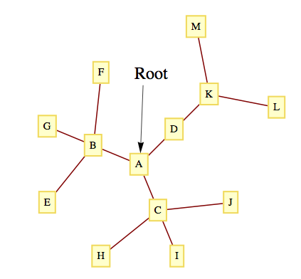
Figure10.3.1.A Rooted TreeList10.3.2.Informal Definition and Terminology
What differentiates rooted trees from undirected trees is that a rooted tree contains a distinguished vertex, called the root. Consider the tree in Figure 10.3.1. Vertex \(A\) has been designated the root of the tree. If we choose any other vertex in the tree, such as \(M\text{,}\) we know that there is a unique path from \(A\) to \(M\text{.}\) The vertices on this path, \((A, D, K, M)\text{,}\) are described in genealogical terms:
\(M\) is a child of \(K\) (so is \(L\))
\(K\) is \(M\)’s parent.
\(A\text{,}\)\(D\text{,}\) and \(K\) are \(M\)’s ancestors.
\(D\text{,}\)\(K\text{,}\) and \(M\) are descendants of \(A\text{.}\)
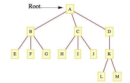
These genealogical relationships are often easier to visualize if the tree is rewritten so that children are positioned below their parents, as in Figure 10.3.3.
With this format, it is easy to see that each vertex in the tree can be thought of as the root of a tree that contains, in addition to itself, all of its descendants. For example, \(D\) is the root of a tree that contains \(D\text{,}\)\(K\text{,}\)\(L\text{,}\) and \(M\text{.}\) Furthermore, \(K\) is the root of a tree that contains \(K\text{,}\)\(L\text{,}\) and \(M\text{.}\) Finally, \(L\) and \(M\) are roots of trees that contain only themselves. From this observation, we can give a formal definition of a rooted tree.
Figure10.3.3.A Rooted Tree, redrawn
One can formally define the genealogical terms above. We define child here since it’s used in our formal definition of a rooted tree and leave the rest of the definitions as an exercise.
Definition10.3.4.Child of a Root.
Given a rooted tree with root \(v\text{,}\) a child of \(v\) is a vertex that is connected to \(v\) by an edge of the tree. We refer to the root as the parent of each of its children.
Definition10.3.5.Rooted Tree.
A single vertex \(v\) with no children is a rooted tree with root \(v\text{.}\)
Recursion: Let \(T_1, T_2,\ldots,T_r\text{,}\)\(r\geq 1\text{,}\) be disjoint rooted trees with roots \(v_1\text{,}\)\(v_2, \ldots \text{,}\)\(v_r\text{,}\) respectively, and let \(v_0\) be a vertex that does not belong to any of these trees. Then a rooted tree, rooted at \(v_0\text{,}\) is obtained by making \(v_0\) the parent of the vertices \(v_1\text{,}\)\(v_2, \ldots\text{,}\) and \(v_r\text{.}\) We call \(T_1, T_2, \ldots, T_r\) subtrees of the larger tree.
The level of a vertex of a rooted tree is the number of edges that separate the vertex from the root. The level of the root is zero. The depth of a tree is the maximum level of the vertices in the tree. The depth of a tree in Figure 10.3.3 is three, which is the level of the vertices \(L\) and \(M\text{.}\) The vertices \(E\text{,}\)\(F\text{,}\)\(G\text{,}\)\(H\text{,}\)\(I\text{,}\)\(J\text{,}\) and \(K\) have level two. \(B\text{,}\)\(C\text{,}\) and \(D\) are at level one and \(A\) has level zero.
One of the keys to working with large amounts of information is to organize it in a consistent, logical way. A data structure is a scheme for organizing data. A simple example of a data structure might be the information a college admissions department might keep on their applicants. Items might look something like this:
A spreadsheet can be used to arrange data in this way. Although a “flat file” structure is often adequate, there are advantages to clustering some the information. For example the applicant information might be broken into four parts: name, contact information, high school, and application data:
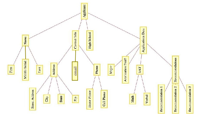
The first item in each ApplicantItem is a list \((FirstName, MiddleInitial, LastName)\text{,}\) with each item in that list being a single field of the original flat file. The third item is simply the single high school item from the flat file. The application data is a list and one of its items, is itself a list with the recommendation data for each recommendation the applicant has.
The organization of this data can be visualized with a rooted tree such as the one in Figure 10.3.8.
Figure10.3.8.Applicant Data in a Rooted Tree
In general, you can represent a data item, \(T\text{,}\) as a rooted tree with \(T\) as the root and a subtree for each field. Those fields that are more than just one item are roots of further subtrees, while individual items have no further children in the tree.
Subsection10.3.2Kruskal’s Algorithm
An alternate algorithm for constructing a minimal spanning tree uses a forest of rooted trees. First we will describe the algorithm in its simplest terms. Afterward, we will describe how rooted trees are used to implement the algorithm. Finally, we will demonstrate the SageMath implementation of the algorithm. In all versions of this algorithm, assume that \(G = (V, E, w)\) is a weighted undirected graph with \(\lvert V\rvert = m\) and \(\lvert E\rvert = n\text{.}\)
Sort the edges of \(G\) in ascending order according to weight. That is,
\begin{equation*}
i \leq j \Leftrightarrow w\left(e_j\right) \leq w\left(e_j\right)\text{.}
\end{equation*}
Go down the list from Step 1 and add edges to a set (initially empty) of edges so that the set does not form a cycle. When an edge that would create a cycle is encountered, ignore it. Continue examining edges until either \(m - 1\) edges have been selected or you have come to the end of the edge list. If \(m - 1\) edges are selected, these edges make up a minimal spanning tree for \(G\text{.}\) If fewer than \(m - 1\) edges are selected, \(G\) is not connected.
Step 1 can be accomplished using one of any number of standard sorting routines. Using the most efficient sorting routine, the time required to perform this step is proportional to \(n \log n\text{.}\) The second step of the algorithm, also of \(n \log n\) time complexity, is the one that uses a forest of rooted trees to test for whether an edge should be added to the spanning set.
Algorithm10.3.10.Kruskal’s Algorithm.
Sort the edges of \(G\) in ascending order according to weight. That is,
\begin{equation*}
i \leq j \Leftrightarrow w\left(e_i \right) \leq w\left(e_j\right)\text{.}
\end{equation*}
Initialize each vertex in V to be the root of its own rooted tree.
Go down the list of edges until either a spanning tree is completed or the edge list has been exhausted. For each edge \(e =\left\{v_1,v_2\right\}\text{,}\) we can determine whether e can be added to the spanning set without forming a cycle by determining whether the root of \({v_1}'s\) tree is equal to the root of \({v_2}'s\) tree. If the two roots are equal, then ignore e. If the roots are different, then we can add e to the spanning set. In addition, we merge the trees that \(v_1\) and \(v_2\) belong to. This is accomplished by either making \({v_1}'s\) root the parent of \({v_2}'s\) root or vice versa.
Note10.3.11.
Since we start the Kruskal’s algorithm with \(m\) trees and each addition of an edge decreases the number of trees by one, we end the algorithm with one rooted tree, provided a spanning tree exists.
The rooted tree that we develop in the algorithm is not the spanning tree itself.
Subsection10.3.3SageMath Note - Implementation of Kruskal’s Algorithm
Kruskal’s algorithm has been implemented in Sage. We illustrate how the spanning tree for a weighted graph in can be generated. First, we create such a graph
We will create a graph using a list of triples of the form \((\text{vertex},\text{vertex}, \text{label})\text{.}\) The \(weighted\) method tells Sage to consider the labels as weights.
Figure10.3.12.Weighed graph, SageMath output
Next, we load the kruskal function and use it to generate the list of edges in a spanning tree of \(G\text{.}\)
To see the resulting tree with the same embedding as \(G\text{,}\) we generate a graph from the spanning tree edges. Next, we set the positions of the vertices to be the same as in the graph. Finally, we plot the tree.
Figure10.3.13.Spanning tree, SageMath output
Exercises10.3.4Exercises
1.
Suppose that an undirected tree has diameter \(d\) and that you would like to select a vertex of the tree as a root so that the resulting rooted tree has the smallest depth possible. How would such a root be selected and what would be the depth of the tree (in terms of \(d\))?
Locate any simple path of length \(d\) and locate the vertex in position \(\lceil d/2\rceil\) on the path. The tree rooted at that vertex will have a depth of \(\lceil d/2\rceil\text{,}\) which is minimal.
2.
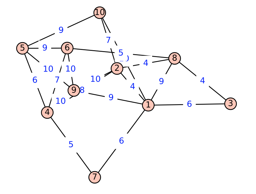
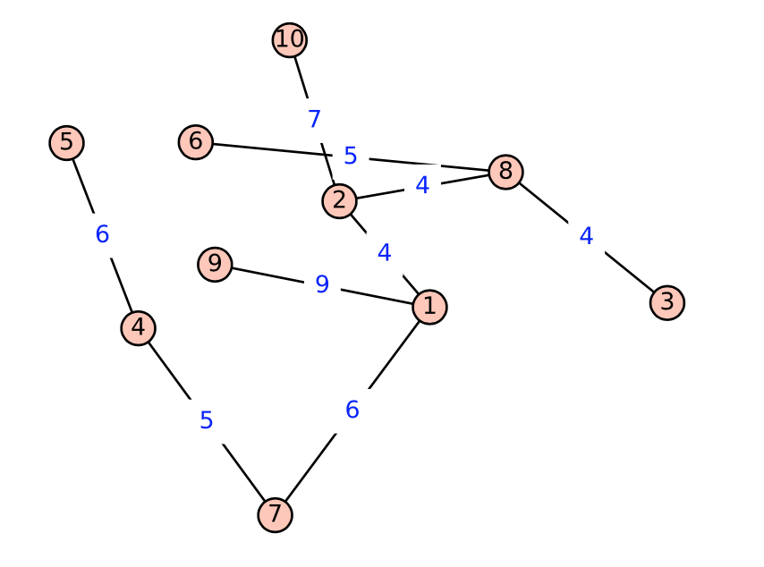
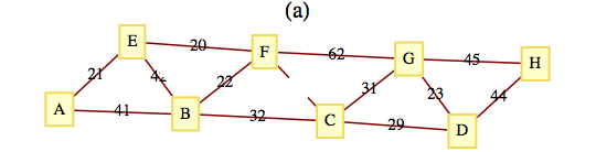
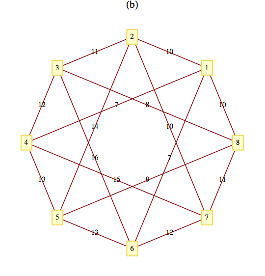
Use Kruskal’s algorithm to find a minimal spanning tree for the following graphs. In addition to the spanning tree, find the final rooted tree in the algorithm. When you merge two trees in the algorithm, make the root with the lower number the root of the new tree.
Figure10.3.14.
Figure10.3.15.
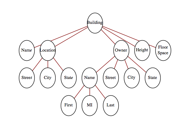
3.
Suppose that information on buildings is arranged in records with five fields: the name of the building, its location, its owner, its height, and its floor space. The location and owner fields are records that include all of the information that you would expect, such as street, city, and state, together with the owner’s name (first, middle, last) in the owner field. Draw a rooted tree to describe this type of record