
Section 12.5 Some Applications
A large and varied number of applications involve computations of powers of matrices. These applications can be found in science, the social sciences, economics, engineering, and, many other areas where mathematics is used. We will consider a few diverse examples the mathematics behind these applications here.
Subsection 12.5.1 Diagonalization
We begin by developing a helpful technique for computing \(A^m\text{,}\) \(m > 1\text{.}\) If \(A\) can be diagonalized, then there is a matrix \(P\) such that \(P^{-1}A P = D\text{,}\) where \(D\) is a diagonal matrix and
\begin{gather}
A^m= P D^m P^{-1} \textrm{ for all } m\geq 1\tag{12.5.1}
\end{gather}
The proof of this identity was an exercise in Section 5.4. The condition that \(D\) be a diagonal matrix is not necessary but when it is, the calculation on the right side is particularly easy to perform. Although the formal proof is done by induction, the reason why it is true is easily seen by writing out an example such as \(m=3\text{:}\)
\begin{equation*}
\begin{split}
A^3 & = \left(P D P^{-1}\right)^3\\
& =\left(P D P^{-1}\right)\left(P D P^{-1}\right)\left(P D P^{-1}\right)\\
&= P D \left(P^{-1}P\right) D \left(P^{-1}P \right)D P^{-1}\quad\textrm{by associativity of matrix multiplication}\\
&= P D I D I D P^{-1}\\
&= P D D D P^{-1}\\
&= P D^3 P^{-1}\\
\end{split}
\end{equation*}
Consider the computation of terms of the Fibonnaci Sequence. Recall that \(F_0= 1, F_1= 1\) and \(F_k= F_{k-1}+F_{k-2}\) for \(k\geq 2\text{.}\)
In order to formulate the calculation in matrix form, we introduced the “dummy equation” \(F_{k-1}= F_{k-1}\) so that now we have two equations
\begin{equation*}
\begin{array}{c}
F_k= F_{k-1}+F_{k-2}\\
F_{k-1}= F_{k-1}\\
\end{array}
\end{equation*}
If \(A = \left(
\begin{array}{cc}
1 & 1 \\
1 & 0 \\
\end{array}
\right)\text{,}\) these two equations can be expressed in matrix form as
\begin{equation*}
\begin{split}
\left(
\begin{array}{c}
F_k \\
F_{k-1} \\
\end{array}
\right) &=\left(
\begin{array}{cc}
1 & 1 \\
1 & 0 \\
\end{array}
\right)\left(
\begin{array}{c}
F_{k-1} \\
F_{k-2} \\
\end{array}
\right) \quad\textrm{ if } k\geq 2\\
&= A \left(
\begin{array}{c}
F_{k-1} \\
F_{k-2} \\
\end{array}
\right)\\
&= A^2\left(
\begin{array}{c}
F_{k-2} \\
F_{k-3} \\
\end{array}
\right) \quad\textrm{ if } k\geq 3\\
& etc.\\
\end{split}
\end{equation*}
We can use induction to prove that if \(k\geq 2\text{,}\)
\begin{equation*}
\left(
\begin{array}{c}
F_k \\
F_{k-1} \\
\end{array}
\right)=A^{k-1} \left(
\begin{array}{c}
1 \\
1 \\
\end{array}
\right)
\end{equation*}
Next, by diagonalizing \(A\) and using the fact that \(A^{m }= P D^m P^{-1}\text{.}\) we can show that
\begin{equation*}
F_k= \frac{1}{\sqrt{5}}\left( \left(\frac{1+\sqrt{5}}{2}\right)^k- \left(\frac{1-\sqrt{5}}{2}\right)^k\right)
\end{equation*}
Some comments on this example:
- An equation of the form \(F_k = a F_{k-1} + b F_{k-2}\) , where \(a\) and \(b\) are given constants, is referred to as a linear homogeneous second-order difference equation. The conditions \(F_0=c_0\) and \(F_1= c_1\) , where \(c_1\) and \(c_2\) are constants, are called initial conditions. Those of you who are familiar with differential equations may recognize that this language parallels what is used in differential equations. Difference (aka recurrence) equations move forward discretely; that is, in a finite number of positive steps. On the other hand, a differential equation moves continuously; that is, takes an infinite number of infinitesimal steps.
- A recurrence relationship of the form \(S_k = a S_{k-1} + b\text{,}\) where \(a\) and \(b\) are constants, is called a first-order difference equation. In order to write out the sequence, we need to know one initial condition. Equations of this type can be solved similarly to the method outlined in the example by introducing the superfluous equation \(1 =0\cdot F_{k-1}+1\) to obtain in matrix equation:\begin{equation*} \left( \begin{array}{c} F_k \\ 1 \\ \end{array} \right)=\left( \begin{array}{cc} a & b \\ 0 & 1 \\ \end{array} \right)\left( \begin{array}{c} S_{k-1} \\ 1 \\ \end{array} \right)\textrm{ }\Rightarrow \left( \begin{array}{c} F_k \\ 1 \\ \end{array} \right)=\left( \begin{array}{cc} a & b \\ 0 & 1 \\ \end{array} \right)^k\left( \begin{array}{c} F_0 \\ 1 \\ \end{array} \right) \end{equation*}
Subsection 12.5.2 Path Counting
In the next example, we apply the following theorem, which can be proven by induction.
Theorem 12.5.2. Path Counting Theorem.
If \(A\) is the adjacency matrix of a graph with vertices \(\{v_1, v_2, \dots,v_n\}\text{,}\) then the entry \(\left(A^k\right)_{ij}\) is the number of paths of length \(k\) from node \(v_i\) to node \(v_j\text{.}\)
Example 12.5.3. Counting Paths with Diagonalization.
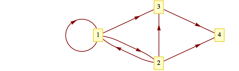
Consider the graph in Figure 12.5.4.

As we saw in Section 6.4, the adjacency matrix of this graph is \(A=\left(
\begin{array}{ccc}
1 & 1 & 0 \\
1 & 0 & 1 \\
0 & 1 & 1 \\
\end{array}
\right)\text{.}\)
Recall that \(A^k\) is the adjacency matrix of the relation \(r^k\text{,}\) where \(r\) is the relation \(\{(a, a), (a, b), (b, a), (b, c), (c, b), (c, c)\}\) of the above graph. Also recall that in computing \(A^k\text{,}\) we used Boolean arithmetic. What happens if we use “regular” arithmetic? If we square \(A\) we get \(A^2 = \left(
\begin{array}{ccc}
2 & 1 & 1 \\
1 & 2 & 1 \\
1 & 1 & 2 \\
\end{array}
\right)\)
How can we interpret this? We note that \(A_{33} = 2\) and that there are two paths of length two from \(c\) (the third node) to \(c\text{.}\) Also, \(A_{13} = 1\text{,}\) and there is one path of length 2 from \(a\) to \(c\text{.}\) The reader should verify these claims by examining the graph.
How do we compute \(A^k\) for possibly large values of \(k\text{?}\) From the discussion at the beginning of this section, we know that \(A^k= P D^kP^{-1}\) if \(A\) is diagonalizable. We leave to the reader to show that \(\lambda = 1, 2,\textrm{ and } -1\) are eigenvalues of \(A\) with eigenvectors
\begin{equation*}
\left(
\begin{array}{c}
1 \\
0 \\
-1 \\
\end{array}
\right),\left(
\begin{array}{c}
1 \\
1 \\
1 \\
\end{array}
\right), \textrm{ and } \left(
\begin{array}{c}
1 \\
-2 \\
1 \\
\end{array}
\right)
\end{equation*}
Then
\begin{equation*}
A^k= P \left(
\begin{array}{ccc}
1 & 0 & 0 \\
0 & 2^k & 0 \\
0 & 0 & (-1)^k \\
\end{array}
\right)P^{-1}
\end{equation*}
where \(P=\left(
\begin{array}{ccc}
1 & 1 & 1 \\
0 & 1 & -2 \\
-1 & 1 & 1 \\
\end{array}
\right)\) and \(P^{-1}=\left(
\begin{array}{ccc}
\frac{1}{2} & 0 & -\frac{1}{2} \\
\frac{1}{3} & \frac{1}{3} & \frac{1}{3} \\
\frac{1}{6} & -\frac{1}{3} & \frac{1}{6} \\
\end{array}
\right)\)
See Exercise 12.5.5.5 of this section for the completion of this example.
Subsection 12.5.3 Matrix Calculus
Example 12.5.5. Matrix Calculus - Exponentials.
Those who have studied calculus recall that the Maclaurin series is a useful way of expressing many common functions. For example, \(e^x=\sum _{k=0}^{\infty } \frac{x^k}{k!}\text{.}\) Indeed, calculators and computers use these series for calculations. Given a polynomial \(f(x)\text{,}\) we defined the matrix-polynomial \(f(A)\) for square matrices in Chapter 5. Hence, we are in a position to describe \(e^A\) for an \(n \times n\) matrix \(A\) as a limit of polynomials, the partial sums of the series. Formally, we write
\begin{equation*}
e^A= I + A + \frac{A^2}{2! }+ \frac{A^3}{3!}+ \cdots = \sum _{k=0}^{\infty } \frac{A^k}{k!}
\end{equation*}
Again we encounter the need to compute high powers of a matrix. Let \(A\) be an \(n\times n\) diagonalizable matrix. Then there exists an invertible \(n\times n\) matrix \(P\) such that \(P^{-1}A P = D\text{,}\) a diagonal matrix, so that
\begin{equation*}
\begin{split}
e^A &=e^{P D P^{-1} }\\
& =\sum _{k=0}^{\infty } \frac{\left(P D P^{-1}\right)^k}{k!} \\
& = P \left(\sum _{k=0}^{\infty } \frac{ D^k}{k!}\right)P^{-1}
\end{split}
\end{equation*}
The infinite sum in the middle of this final expression can be easily evaluated if \(D\) is diagonal. All entries of powers off the diagonal are zero and the \(i^{\textrm{ th}}\) entry of the diagonal is
\begin{equation*}
\left(\sum _{k=0}^{\infty } \frac{ D^k}{k!}\right){}_{i i}=\sum _{k=0}^{\infty } \frac{ D_{i i}{}^k}{k!}= e^{D_{ii}}
\end{equation*}
For example, if \(A=\left(
\begin{array}{cc}
2 & 1 \\
2 & 3 \\
\end{array}
\right)\text{,}\) the first matrix we diagonalized in Section 12.3, we found that \(P =\left(
\begin{array}{cc}
1 & 1 \\
-1 & 2 \\
\end{array}
\right)\) and \(D= \left(
\begin{array}{cc}
1 & 0 \\
0 & 4 \\
\end{array}
\right)\text{.}\)
Therefore,
\begin{equation*}
\begin{split}
e^A &=\left(
\begin{array}{cc}
1 & 1 \\
-1 & 2 \\
\end{array}
\right) \left(
\begin{array}{cc}
e & 0 \\
0 & e^4 \\
\end{array}
\right) \left(
\begin{array}{cc}
\frac{2}{3} & -\frac{1}{3} \\
\frac{1}{3} & \frac{1}{3} \\
\end{array}
\right)\\
&= \left(
\begin{array}{cc}
\frac{2 e}{3}+\frac{e^4}{3} & -\frac{e}{3}+\frac{e^4}{3} \\
-\frac{2 e}{3}+\frac{2 e^4}{3} & \frac{e}{3}+\frac{2 e^4}{3} \\
\end{array}
\right)\\
& \approx \left(
\begin{array}{cc}
20.0116 & 17.2933 \\
34.5866 & 37.3049 \\
\end{array}
\right)
\end{split}
\end{equation*}
Remark 12.5.6.
Many of the ideas of calculus can be developed using matrices. For example, if \(A(t) = \left(
\begin{array}{cc}
t^3 & 3 t^2+8t \\
e^t & 2 \\
\end{array}
\right)\) then \(\frac{d A(t)}{d t}=\left(
\begin{array}{cc}
3 t^2 & 6 t+8 \\
e^t & 0 \\
\end{array}
\right)\)
Many of the basic formulas in calculus are true in matrix calculus. For example,
\begin{equation*}
\frac{d (A(t)+B(t))}{d t} = \frac{d A(t)}{d t}+ \frac{d B(t)}{d t}
\end{equation*}
and if \(A\) is a constant matrix,
\begin{equation*}
\frac{d e^{A t}}{d t}= A e^{A t}
\end{equation*}
Matrix calculus can be used to solve systems of differential equations in a similar manner to the procedure used in ordinary differential equations.
Subsection 12.5.4 SageMath Note - Matrix Exponential
Sage’s matrix exponential method is
exp.Exercises 12.5.5 Exercises
1.
- Write out all the details of Example 12.5.1 to show that the formula for \(F_k\) given in the text is correct.
- Use induction to prove the assertion made in the example that \(\left( \begin{array}{c} F_k \\ F_{k-1} \\ \end{array} \right)=A^{k-1} \left( \begin{array}{c} 1 \\ 1 \\ \end{array} \right)\)
2.
- Do Example 8.3.14 using the method outlined in Example 12.5.1. Note that the terminology characteristic equation, characteristic polynomial, and so on, introduced in Chapter 8, comes from the language of matrix algebra,
- What is the significance of Algorithm 8.3.12, part c, with respect to this section?
3.
Solve \(S(k) = 5S(k - 1) + 4\text{,}\) with \(S(0) = 0\text{,}\) using the method of this section.
4.
How many paths are there of length 6 from vertex 1 to vertex 3 in Figure 12.5.7? How many paths from vertex 2 to vertex 2 of length 6 are there?
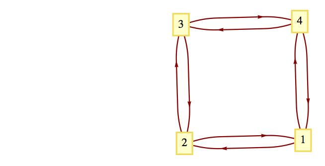
Hint.
The characteristic polynomial of the adjacency matrix is \(\lambda ^4 - 4 \lambda^2\text{.}\)
5.
Regarding Example 12.5.3,
- Use matrices to determine the number of paths of length 1 that exist from vertex \(a\) to each of the vertices in the given graph. Verify using the graph. Do the same for vertices \(b\) and \(c\text{.}\)
- Verify all the details provided in the example.
- Use matrices to determine the number of paths of length 4 there between each pair of nodes in the graph. Verify your results using the graph.
Answer.
- Since \(A=A^1= \left( \begin{array}{ccc} 1 & 1 & 0 \\ 1 & 0 & 1 \\ 0 & 1 & 1 \\ \end{array} \right)\text{,}\) there are 0 paths of length 1 from: node c to node a, node b to node b, and node a to node c; and there is 1 path of length 1 for every other pair of nodes.
-
The characteristic polynomial is \(\lvert A-c I\rvert = \left| \begin{array}{ccc} 1-c & 1 & 0 \\ 1 & -c & 1 \\ 0 & 1 & 1-c \\ \end{array} \right| = -c^3+2 c^2+c-2\)Solving the characteristic equation \(-c^3+2 c^2+c-2=0\) we find solutions 1, 2, and -1.If \(c=1\text{,}\) we find the associated eigenvector by finding a nonzero solution to \(\left( \begin{array}{ccc} 0 & 1 & 0 \\ 1 & -1 & 1 \\ 0 & 1 & 0 \\ \end{array} \right)\left( \begin{array}{c} x_1 \\ x_2 \\ x_3 \\ \end{array} \right)=\left( \begin{array}{c} 0 \\ 0 \\ 0 \\ \end{array} \right)\) One of these, which will be the first column of \(P\text{,}\) is \(\left( \begin{array}{c} 1 \\ 0 \\ -1 \\ \end{array} \right)\)If \(c=2\text{,}\) the system \(\left( \begin{array}{ccc} -1 & 1 & 0 \\ 1 & -2 & 1 \\ 0 & 1 & -1 \\ \end{array} \right)\left( \begin{array}{c} x_1 \\ x_2 \\ x_3 \\ \end{array} \right)=\left( \begin{array}{c} 0 \\ 0 \\ 0 \\ \end{array} \right)\) yields eigenvectors, including \(\left( \begin{array}{c} 1 \\ 1 \\ 1 \\ \end{array} \right)\text{,}\) which will be the second column of \(P\text{.}\)If \(c = -1\text{,}\) then the system determining the eigenvectors is \(\left( \begin{array}{ccc} 2 & 1 & 0 \\ 1 & 1 & 1 \\ 0 & 1 & 2 \\ \end{array} \right)\left( \begin{array}{c} x_1 \\ x_2 \\ x_3 \\ \end{array} \right)=\left( \begin{array}{c} 0 \\ 0 \\ 0 \\ \end{array} \right)\) and we can select \(\left( \begin{array}{c} 1 \\ -2 \\ 1 \\ \end{array} \right)\text{,}\) although any nonzero multiple of this vector could be the third column of \(P\text{.}\)
-
Assembling the results of part (b) we have \(P=\left( \begin{array}{ccc} 1 & 1 & 1 \\ 0 & 1 & -2 \\ -1 & 1 & 1 \\ \end{array} \right)\) .\begin{equation*} \begin{split} A^4 & = P \left( \begin{array}{ccc} 1^4 & 0 & 0 \\ 0 & 2^4 & 0 \\ 0 & 0 & (-1)^{4 } \\ \end{array} \right)P^{-1}= P \left( \begin{array}{ccc} 1 & 0 & 0 \\ 0 & 16 & 0 \\ 0 & 0 & 1 \\ \end{array} \right)P^{-1}\\ &=\left( \begin{array}{ccc} 1 & 16 & 1 \\ 0 & 16 & -2 \\ -1 & 16 & 1 \\ \end{array} \right)\left( \begin{array}{ccc} \frac{1}{2} & 0 & -\frac{1}{2} \\ \frac{1}{3} & \frac{1}{3} & \frac{1}{3} \\ \frac{1}{6} & -\frac{1}{3} & \frac{1}{6} \\ \end{array} \right)\\ &=\left( \begin{array}{ccc} 6 & 5 & 5 \\ 5 & 6 & 5 \\ 5 & 5 & 6 \\ \end{array} \right)\\ \end{split} \end{equation*}Hence there are five different paths of length 4 between distinct vertices, and six different paths that start and end at the same vertex. The reader can verify these facts from Figure 12.5.4
6.
Let \(A =\left(
\begin{array}{cc}
2 & -1 \\
-1 & 2 \\
\end{array}
\right)\)
- Find \(e^A\)
- Recall that \(\sin x = \sum _{k=0}^{\infty } \frac{(-1)^k x^k}{(2 k+1)!}\) and compute \(\sin A\text{.}\)
- Formulate a reasonable definition of the natural logarithm of a matrix and compute \(\ln A\text{.}\)
7.
We noted in Chapter 5 that since matrix algebra is not commutative under multiplication, certain difficulties arise. Let \(A=\left(
\begin{array}{cc}
1 & 1 \\
0 & 0 \\
\end{array}
\right)\) and \(B=\left(
\begin{array}{cc}
0 & 0 \\
0 & 2 \\
\end{array}
\right)\text{.}\)
- Compute \(e^A\text{,}\) \(e^B\text{,}\) and \(e^{A+B}\text{.}\) Compare \(e^A e^{B}\text{,}\) \(e^B e^A\) and \(e^{A+B}\) .
- Show that if \(\pmb{0}\) is the \(2\times 2\) zero matrix, then \(e^{\pmb{0}}= I\text{.}\)
- Prove that if \(A\) and \(B\) are two matrices that do commute, then \(e^{A+B}=e^Ae^B\text{,}\) thereby proving that \(e^A\) and \(e^B\) commute.
- Prove that for any matrix \(A\text{,}\) \(\left(e^A\right)^{-1}= e^{-A}\text{.}\)
Answer.
- \(e^A=\left( \begin{array}{cc} e & e \\ 0 & 0 \\ \end{array} \right)\) , \(e^B=\left( \begin{array}{cc} 0 & 0 \\ 0 & e^2 \\ \end{array} \right)\text{,}\) and \(e^{A+B}=\left( \begin{array}{cc} e & e^2-e \\ 0 & e^2 \\ \end{array} \right)\)
- Let \(\pmb{0}\) be the zero matrix, \(e^{\pmb{0}}=I + \pmb{0}+\frac{\pmb{0}^2}{2}+\frac{\pmb{0}^3}{6}+\ldots =I\) .
- Assume that \(A\) and \(B\) commute. We will examine the first few terms in the product \(e^A e^B\text{.}\) The pattern that is established does continue in general. In what follows, it is important that \(A B = B A\text{.}\) For example, in the last step, \((A+B)^2\) expands to \(A^2+A B + B A + B^2\text{,}\) not \(A^2+ 2 A B + B^2\text{,}\) if we can’t assume commutativity.\begin{equation*} \begin{split} e^Ae^B &= \left(\sum _{k=0}^{\infty } \frac{A^k}{k!}\right) \left(\sum _{k=0}^{\infty } \frac{B^k}{k!}\right)\\ & =\left(I + A+\frac{A^2}{2}+ \frac{A^3}{6}+ \cdots \right)\left(I +B+\frac{B^2}{2}+ \frac{B^3}{6}+ \cdots \right)\\ &= I + A + B+ \frac{A^2}{2}+ A B + \frac{B^2}{2}+\frac{A^3}{6}+ \frac{A^2B}{2}+\frac{A B^2}{2}+ \frac{B^3}{6}+\cdots \\ &= I + (A+B) + \frac{1}{2}\left(A^2+ 2 A B + B^2\right)+ \frac{1}{6}\left(A^3+ 3A^2B+ 3A B^2+ B^3\right)+\cdots \\ &=I + (A+B)+ \frac{1}{2}(A+B)^2+ \frac{1}{6}(A+B)^3+\cdots \\ & =e^{A+B}\\ \end{split} \end{equation*}
- Since \(A\) and \(-A\) commute, we can apply part d;\begin{equation*} e^Ae^{-A} = e^{A+(-A)} =e^{\pmb{0}} =I \end{equation*}
8.
Another observation for adjacency matrices: For the matrix in Example 12.5.3, note that the sum of the elements in the row corresponding to the node \(a\) (that is, the first row) gives the outdegree of \(a\text{.}\) Similarly, the sum of the elements in any given column gives the indegree of the node corresponding to that column.
- Using the matrix \(A\) of Example 12.5.3, find the outdegree and the indegree of each node. Verify by the graph.
- Repeat part (a) for the directed graphs in Figure 12.5.8.
