In this section, we will introduce the concept of a language. Languages are subsets of a certain type of monoid, the free monoid over an alphabet. After defining a free monoid, we will discuss languages and some of the basic problems relating to them. We will also discuss the common ways in which languages are defined.
Let \(A\) be a nonempty set, which we will call an alphabet. Our primary interest will be in the case where \(A\) is finite; however, \(A\) could be infinite for most of the situations that we will describe. The elements of \(A\) are called letters or symbols. Among the alphabets that we will use are \(B=\{0,1\}\text{,}\) and the set of ASCII (American Standard Code for Information Interchange) characters, which we symbolize as \(ASCII\text{.}\)
Definition14.2.1.Strings over an Alphabet.
A string of length \(n\text{,}\)\(n \geqslant 1\) over alphabet \(A\) is a sequence of \(n\) letters from \(A\text{:}\)\(a_1a_2\ldots a_n\text{.}\) The null string, \(\lambda\text{,}\) is defined as the string of length zero containing no letters. The set of strings of length \(n\) over \(A\) is denoted by \(A^n\text{.}\) The set of all strings over \(A\) is denoted \(A^*\text{.}\)
Note14.2.2.
If the length of string \(s\) is \(n\text{,}\) we write \(\lvert s \rvert =n\text{.}\)
The null string is not the same as the empty set, although they are similar in many ways. \(A^0 = \{\lambda\}\text{.}\)
\(A^*=A^0\cup A^1\cup A^2\cup A^3\cup \cdots \textrm{ and if } i\neq j,A^i\cap A^j=\emptyset\text{;}\) that is, \(\{A^0,A^1,A^2,A^3,\ldots \}\) is a partition of \(A^*\text{.}\)
An element of \(A\) can appear any number of times in a string.
Case 1. Given the alphabet \(B=\{0,1\}\text{,}\) we can define a bijection from the positive integers into \(B^*\text{.}\) Each positive integer has a binary expansion \(d_kd_{k-1}\cdots d_1d_0\text{,}\) where each \(d_j\) is 0 or 1 and \(d_k=1\text{.}\) If \(n\) has such a binary expansion, then \(2^k \leq n\leq 2^{k+1}\text{.}\) We define \(f:\mathbb{P}\to B^*\) by \(f(n)=f\left(d_kd_{k-1}\cdots d_1d_0\right)=d_{k-1}\cdots d_1d_0,\) where \(f(1)=\lambda\text{.}\) Every one of the \(2^k\) strings of length \(k\) are the images of exactly one of the integers between \(2^k\textrm{ and } 2^{k+1}-1.\) From its definition, \(f\) is clearly a bijection; therefore, \(B^*\) is countable.
Case 2: \(A\) is Finite. We will describe how this case is handled with an example first and then give the general proof. If \(A=\{a,b,c,d,e\}\text{,}\) then we can code the letters in \(A\) into strings from \(B^3\text{.}\) One of the coding schemes (there are many) is \(a\leftrightarrow 000, b\leftrightarrow
001, c\leftrightarrow 010, d\leftrightarrow 011, \textrm{ and } e\leftrightarrow 100\text{.}\) Now every string in \(A^*\) corresponds to a different string in \(B^*\text{;}\) for example, \(ace\text{.}\) would correspond with \(000010100\text{.}\) The cardinality of \(A^*\) is equal to the cardinality of the set of strings that can be obtained from this encoding system. The possible coded strings must be countable, since they are a subset of a countable set, \(B^*\text{.}\) Therefore, \(A^*\) is countable.
If \(\lvert A\rvert =m\text{,}\) then the letters in \(A\) can be coded using a set of fixed-length strings from \(B^*\text{.}\) If \(2^{k-1} < m \leq 2^k\text{,}\) then there are at least as many strings of length \(k\) in \(B^k\) as there are letters in \(A\text{.}\) Now we can associate each letter in \(A\) with with a different element of \(B^k\text{.}\) Then any string in \(A^*\text{.}\) corresponds to a string in \(B^*\text{.}\) By the same reasoning as in the example above, \(A^*\) is countable.
Case 3: \(A\) is Countably Infinite. We will leave this case as an exercise.
Definition14.2.4.Concatenation.
Let \(a=a_1a_2\cdots a_m\) and \(b=b_1b_2\cdots b_n\) be strings of length \(m\) and \(n\text{,}\) respectively. The concatenation of \(a\) with \(b\text{,}\)\(a+b\text{,}\) is the string \(a_1a_2\cdots a_mb_1b_2\cdots b_n\) of length \(m+n\text{.}\)
There are several symbols that are used for concatenation. We chose to use the one that is also used in Python and SageMath.
The set of strings over any alphabet is a monoid under concatenation.
Note14.2.5.
The null string is the identity element of \([A^*; +]\text{.}\) Henceforth, we will denote the monoid of strings over \(A\) by \(A^*\text{.}\)
Concatenation is noncommutative, provided \(\lvert A\rvert > 1\text{.}\)
If \(\lvert A_1 \rvert = \lvert A_2 \rvert\text{,}\) then the monoids \(A_1^*\) and \(A_2^*\) are isomorphic. An isomorphism can be defined using any bijection \(f:A_1\to A_2\text{.}\) If \(a=a_1a_2\cdots a_n \in A_1^*\text{,}\)\(f^*(a)=(f(a_1)f(a_2)\cdots f(a_n))\) defines a bijection from \(A_1^*\) into \(A_2^*\text{.}\) We will leave it to the reader to prove that for all \(a,b,\in A_1^*,f^*(a+b)=f^*(a)+f^*(b)\text{.}\)
The languages of the world, English, German, Russian, Chinese, and so forth, are called natural languages. In order to communicate in writing in any one of them, you must first know the letters of the alphabet and then know how to combine the letters in meaningful ways. A formal language is an abstraction of this situation.
Definition14.2.6.Formal Language.
If \(A\) is an alphabet, a formal language over \(A\) is a subset of \(A^*\text{.}\)
English can be thought of as a language over of letters \(A,B,\cdots Z\text{,}\) both upper and lower case, and other special symbols, such as punctuation marks and the blank. Exactly what subset of the strings over this alphabet defines the English language is difficult to pin down exactly. This is a characteristic of natural languages that we try to avoid with formal languages.
The set of all ASCII stream files can be defined in terms of a language over ASCII. An ASCII stream file is a sequence of zero or more lines followed by an end-of-file symbol. A line is defined as a sequence of ASCII characters that ends with the a “new line” character. The end-of-file symbol is system-dependent.
The set of all syntactically correct expressions in any computer language is a language over the set of ASCII strings.
A few languages over \(B\) are
\(\displaystyle L_1=\{s\in B^* \mid s \textrm{ has exactly as many 1's as it has 0's}\}\)
\(\displaystyle L_2=\{1+s+0 \mid s\in B^*\}\)
\(L_3=\langle 0,01\rangle\) = the submonoid of \(B^*\) generated by \(\{0,01\}\text{.}\)
Investigation14.2.1.Two Fundamental Problems: Recognition and Generation.
The generation and recognition problems are basic to computer programming. Given a language, \(L\text{,}\) the programmer must know how to write (or generate) a syntactically correct program that solves a problem. On the other hand, the compiler must be written to recognize whether a program contains any syntax errors.
Given a formal language over alphabet \(A\text{,}\) the Recognition Problem is to design an algorithm that determines the truth of \(s\in L\) in a finite number of steps for all \(s\in A^*\text{.}\) Any such algorithm is called a recognition algorithm.
Definition14.2.9.Recursive Language.
A language is recursive if there exists a recognition algorithm for it.
The language of syntactically correct propositions over set of propositional variables expressions is recursive.
The three languages in 7(d) are all recursive. Recognition algorithms for \(L_1\) and \(L_2\) should be easy for you to imagine. The reason a recognition algorithm for \(L_3\) might not be obvious is that the definition of \(L_3\) is more cryptic. It doesn’t tell us what belongs to \(L_3\text{,}\) just what can be used to create strings in \(L_3\text{.}\) This is how many languages are defined. With a second description of \(L_3\text{,}\) we can easily design a recognition algorithm. You can prove that
\begin{equation*}
L_3=\{s\in B^* \mid s=\lambda \textrm{ or } s \textrm{ starts with a 0 and has no consecutive 1's}\}\text{.}
\end{equation*}
Design an algorithm that generates or produces any string in \(L\text{.}\) Here we presume that \(A\) is either finite or countably infinite; hence, \(A^*\) is countable by Theorem 14.2.3, and \(L \subseteq A^*\) must be countable. Therefore, the generation of \(L\) amounts to creating a list of strings in \(L\text{.}\) The list may be either finite or infinite, and you must be able to show that every string in \(L\) appears somewhere in the list.
Theorem14.2.12.Recursive implies Generating.
If \(A\) is countable, then there exists a generating algorithm for \(A^*\text{.}\)
If \(L\) is a recursive language over a countable alphabet, then there exists a generating algorithm for \(L\text{.}\)
Part (a) follows from the fact that \(A^*\) is countable; therefore, there exists a complete list of strings in \(A^*\text{.}\)
To generate all strings of \(L\text{,}\) start with a list of all strings in \(A^*\) and an empty list, \(W\text{,}\) of strings in \(L\text{.}\) For each string \(s\text{,}\) use a recognition algorithm (one exists since \(L\) is recursive) to determine whether \(s\in L\text{.}\) If \(s \in L\text{,}\) add it to \(W\text{;}\) otherwise “throw it out.” Then go to the next string in the list of \(A^*\text{.}\)
Since all of the languages in 7(d) are recursive, they must have generating algorithms. The one given in the proof of Theorem 14.2.12 is not usually the most efficient. You could probably design more efficient generating algorithms for \(L_2\) and \(L_3\text{;}\) however, a better generating algorithm for \(L_1\) is not quite so obvious.
The recognition and generation problems can vary in difficulty depending on how a language is defined and what sort of algorithms we allow ourselves to use. This is not to say that the means by which a language is defined determines whether it is recursive. It just means that the truth of the statement “\(L\) is recursive” may be more difficult to determine with one definition than with another. We will close this section with a discussion of grammars, which are standard forms of definition for a language. When we restrict ourselves to only certain types of algorithms, we can affect our ability to determine whether \(s\in L\) is true. In defining a recursive language, we do not restrict ourselves in any way in regard to the type of algorithm that will be used. In the next section, we will consider machines called finite automata, which can only perform simple algorithms.
One common way of defining a language is by means of a phrase structure grammar (or grammar, for short). The set of strings that can be produced using set of grammar rules is called a phrase structure language.
We can define the set of all strings over \(B\) for which all 0’s precede all 1’s as follows. Define the starting symbol \(S\) and establish rules that \(S\) can be replaced with any of the following: \(\lambda\text{,}\)\(0S\text{,}\) or \(S1\text{.}\) These replacement rules are usually called production rules. They are usually written in the format \(S\to \lambda\text{,}\)\(S\to 0S\text{,}\) and \(S\to S1\text{.}\) Now define \(L\) to be the set of all strings that can be produced by starting with \(S\) and applying the production rules until \(S\) no longer appears. The strings in \(L\) are exactly the ones that are described above.
Definition14.2.15.Phrase Structure Grammar.
A phrase structure grammar consists of four components:
A nonempty finite set of terminal characters, \(T\text{.}\) If the grammar is defining a language over \(A\text{,}\)\(T\) is a subset of \(A^*\text{.}\)
A finite set of nonterminal characters, \(N\text{.}\)
A starting symbol, \(S\in N\text{.}\)
A finite set of production rules, each of the form \(X\to Y\text{,}\) where \(X\) and \(Y\) are strings over \(A\cup N\) such that \(X\neq Y\) and \(X\) contains at least one nonterminal symbol.
If \(G\) is a phrase structure grammar, \(L(G)\) is the set of strings that can be produced by starting with \(S\) and applying the production rules a finite number of times until no nonterminal characters remain. If a language can be defined by a phrase structure grammar, then it is called a phrase structure language.
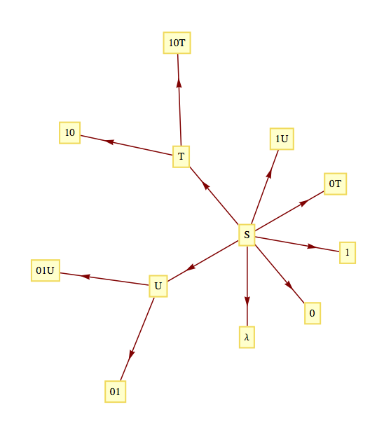
Figure14.2.17.Production rules for the language of alternating 0’s and 1’s
We can verify that a string such as 10101 belongs to the language by starting with \(S\) and producing 10101 using the production rules a finite number of times: \(S\to 1U\to 101U\to 10101\text{.}\)
Terminal symbols = all letters of the alphabet (both upper and lower case), digits 0 through 9, and underscore
Nonterminal symbols: \(\{I, X\}\text{,}\)
Starting symbol: \(I\)
Production rules: \(I \to \alpha\text{,}\) where \(\alpha\) is any letter, \(I \to \alpha+X\) for any letter \(\alpha\text{,}\)\(X\to X+\beta\) for any letter, digit or underscore, \(\beta\text{,}\) and \(X \to \beta\) for any letter, digit or underscore, \(\beta\text{.}\) There are a total of \(52+52+63+63=230\) production rules for this grammar. The language \(L(G)\) consists of all valid SageMath variable names.
Backus-Naur form (BNF) is a popular alternate form of defining the production rules in a grammar. If the production rules \(A\to B_1, A\to B_2,\ldots A\to B_n\) are part of a grammar, they would be written in BNF as \(A ::=B_1 \mid B_2\mid \cdots \mid B_n\text{.}\) The symbol \(\mid\) in BNF is read as “or” while the \(::=\) is read as “is defined as.” Additional notations of BNF are that \(\{x\}\text{,}\) represents zero or more repetitions of \(x\) and \([y]\) means that \(y\) is optional.
A BNF version of the production rules for a SageMath variable, \(I\text{,}\) is
An arithmetic expression can be defined in BNF. For simplicity, we will consider only expressions obtained using addition and multiplication of integers. The terminal symbols are (,),+,*, -, and the digits 0 through 9. The nonterminal symbols are \(E\) (for expression), \(T\) (term), \(F\) (factor), and \(N\) (number). The starting symbol is \(E\text{.}\) Production rules are
\begin{equation*}
\begin{array}{c}
E\text ::=E+T \mid T\\
T ::=T * F \mid F\\
F ::=(E)\mid N\\
N ::=[-]\textrm{digit} \{\textrm{digit}\}\\
\\
\end{array}\text{.}
\end{equation*}
One particularly simple type of phrase structure grammar is the regular grammar.
Definition14.2.21.Regular Grammar.
A regular (right-hand form) grammar is a grammar whose production rules are all of the form \(A\to t\) and \(A\to tB\text{,}\) where \(A\) and \(B\) are nonterminal and \(t\) is terminal. A left-hand form grammar allows only \(A \to t\) and \(A\to Bt\text{.}\) A language that has a regular phrase structure language is called a regular language.
The set of Sage variable names is a regular language since the grammar by which we defined the set is a regular grammar.
The language of all strings for which all 0’s precede all 1’s (Example 14.2.14) is regular; however, the grammar by which we defined this set is not regular. Can you define these strings with a regular grammar?
The language of arithmetic expressions is not regular.
ExercisesExercises
1.
If a computer is being designed to operate with a character set of 350 symbols, how many bits must be reserved for each character? Assume each character will use the same number of bits.
For a character set of 350 symbols, the number of bits needed for each character is the smallest \(n\) such that \(2^n\) is greater than or equal to 350. Since \(2^9= 512 > 350 > 2^8\text{,}\) 9 bits are needed,
\(2^{12}=4096 >3500> 2^{11}\text{;}\) therefore, 12 bits are needed.
2.
It was pointed out in the text that the null string and the null set are different. The former is a string and the latter is a set, two different kinds of objects. Discuss how the two are similar.
3.
What sets of strings are defined by the following grammar?
Terminal symbols: \(\lambda\) , 0 and 1
Nonterminal symbols: \(S\) and \(E\)
Starting symbol: \(S\)
Production rules: \(S\to 0S0, S \to 1S1, S\to E, E \to \lambda, E\to 0, E\to 1\)
Terminal symbols: The null string, 0, and 1. Nonterminal symbols: \(S\text{,}\)\(E\text{.}\) Starting symbol: \(S\text{.}\) Production rules: \(S\to 00S\text{,}\)\(S\to 01S\text{,}\)\(S\to 10S\text{,}\)\(S\to 11S\text{,}\)\(S\to E\text{,}\)\(E\to 0\text{,}\)\(E\to 1\) This is a regular grammar.
Terminal symbols: The null string, 0, and 1. Nonterminal symbols: \(S\text{,}\)\(A\text{,}\)\(B\text{,}\)\(C\) Starting symbol: \(S\) Production rules: \(S \to 0A\text{,}\)\(S \to 1A\text{,}\)\(S \to \lambda\) , \(A \to 0B\text{,}\)\(A \to 1B\text{,}\)\(A \to \lambda\text{,}\)\(B \to 0C\text{,}\)\(B \to 1C\text{,}\)\(B \to A\text{,}\)\(C \to 0\text{,}\)\(C \to 1\text{,}\)\(C \to \lambda\) This is a regular grammar.
See Exercise 3. This language is not regular.
6.
Define the following languages over \(B\) with phrase structure grammars. Which of these languages are regular?
The strings with more 0’s than 1’s.
The strings with an even number of 1’s.
The strings for which all 0’s precede all 1’s.
7.
Prove that if a language over \(A\) is recursive, then its complement is also recursive.
If \(s\) is in \(A^*\) and \(L\) is recursive, we can answer the question “Is s in \(L^c\text{?}\)” by negating the answer to “Is \(s\) in \(L\text{?}\)”
8.
Use BNF to define the grammars in Exercises 3 and 4.
9.
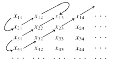
Prove that if \(X_1, X_2, \ldots\)is a countable sequence of countable sets, the union of these sets, \(\underset{i=1}{\overset{\infty }{\cup}}X_i\) is countable.
Using the fact that the countable union of countable sets is countable, prove that if \(A\) is countable, then \(A^*\) is countable.
List the elements of each set \(X_i\) in a sequence \(x_{i 1}\text{,}\)\(x_{i 2}\text{,}\)\(x_{i 3}\ldots\) . Then draw arrows as shown below and list the elements of the union in order established by this pattern: \(x_{11}\text{,}\)\(x_{21}\text{,}\)\(x_{12}\text{,}\)\(x_{13}\text{,}\)\(x_{22}\text{,}\)\(x_{31}\text{,}\)\(x_{41}\text{,}\)\(x_{32}\text{,}\)\(x_{23}\text{,}\)\(x_{14}\text{,}\)\(x_{15}\ldots \text{,}\)
Each of the sets \(A^1\) , \(A^2\) , \(A^3, \ldots\text{,}\) are countable and \(A^*\) is the union of these sets; hence \(A^*\) is countable.